fabric-iq
Part 1: Build a live pharma cold-chain monitor in Microsoft Fabric Real-Time Intelligence, the Eventstream-to-KQL pipeline that scores every reading
A batch of insulin was ruined on a truck that never once got warm, and nobody noticed for three weeks. Part 1 builds the live half in Real-Time Intelligence, from CSV to a stream to a KQL layer that scores every reading against each batch's own safe band.
Batch AUR-2207 left the Aurora Pharma plant in Hyderabad at 4:30 AM. Inside the truck were 1,549 vials of insulin, worth about 22,800 dollars.
It reached the clinic in Warangal before lunch. The insulin was ruined.
Insulin has to stay between 2°C and 8°C. Above 8°C it spoils. Below 2°C it freezes, and frozen insulin does not recover when it thaws. The vial still looks fine. The medicine inside is gone.
So the safe range has two edges. A ceiling at 8°C, and a floor at 2°C. The refrigerated relay that has to hold that range, from the plant through every truck and depot to the clinic, is called the cold chain.
Almost every cold chain alarm watches the ceiling. Go above 8°C and someone gets a message. There is usually no rule at all for the floor.
There is a reason for that, and it is not stupidity. Cold chain exists to keep things cold, so heat is the failure everyone pictures. A cooling unit doing its job a little too well does not feel like a fault.
AUR-2207 was on the road for five and a half hours. The warmest reading in all of it was -19.9°C.
Read that again. The truck was not slightly too cold. It ran about 22 degrees below the floor for 330 minutes, which was every minute of the journey, and no alarm said a word. The alarm was only ever looking up.
| Temperature | What it means for insulin | Does an alarm watch this? |
|---|---|---|
| Above 8°C | Spoils | Yes, almost always |
| 2°C to 8°C | Safe | n/a |
| Below 2°C | Freezes, and cannot be saved | Usually not |
| -20.5°C to -19.9°C, where AUR-2207 spent its whole trip | Frozen solid | No |
Here is how it happened
Aurora ships two kinds of product. Chilled ones like insulin, which ride at 5°C. And a frozen vaccine, which rides at -20°C.
The shipping paperwork for every load has one field for the target temperature. On AUR-2207's paperwork, that field said -20°C. It was the setting for the frozen vaccine, on a truck full of insulin.
Nobody questioned it. The first driver set his unit to -20°C and drove the two hours to the Hyderabad depot. The load was moved to a second truck. That driver read the same paperwork, set the same number, and drove on to Warangal.
The cooling unit was not broken. Neither was the second one. They worked perfectly. They held -20°C for five and a half hours, exactly as instructed, and froze 1,549 vials of insulin on the way.
The alarm watched for heat. The damage came from cold. And the thing that was wrong was not the machine. It was a number on a form.
The part that costs more than the insulin
Nobody noticed for three weeks.
Frozen insulin looks exactly like good insulin. The vial is clear. The label is fine. The seal is intact. A driver cannot see the problem. A pharmacist cannot see it. A patient injecting it cannot see it.
The batch was caught during a routine review of the temperature logs, and only because someone read them line by line. By then the vials were already in clinic refrigerators.
This is not a hypothetical risk. A clinic in Sydney stored vaccines outside their safe range and more than 1,000 patients had to be contacted and vaccinated again.
So the 22,800 dollars is the small number. The real cost is a recall, a regulator asking questions, and a thousand people who trusted a medicine that could not work.
Which leads to the question this whole article is built to answer.
Priya runs quality at the Hyderabad plant. Every morning she needs to know one thing:
Which batches on the road right now are in trouble, and where are they?
Not last month. Not after someone reads the logs line by line. Right now, while the trucks are still moving and the medicine can still be saved.
The rule almost everyone writes
Priya has the data. Aurora runs twelve refrigerated trucks. The shipping industry calls a refrigerated truck a reefer, and that word shows up in file and table names all through this build. Every truck reports its temperature every few minutes. So the answer should be easy: build an alarm.
First attempt: alert when the temperature goes above 8°C.
It fires on 9 of the 12 trucks.
Nothing is broken. Trucks open their doors. Warm air gets in for a few minutes, the temperature jumps, the alarm goes off. This happens at every stop, every day.
After three days, someone mutes the channel.
Second attempt: alert only when the temperature stays above 8°C for 45 minutes.
Now it fires on 2 trucks in ten days. The noise is gone.
That feels like success. It is not.
This rule never sees AUR-2207, because AUR-2207 was never warm.
It also misses AUR-2211, and that one needs a word of background.
No medicine is ruined by a door opening for four minutes. So each product gets a small allowance: a total number of minutes it may spend outside its safe range across a whole journey, before the batch has to be pulled and inspected. Time outside the safe range is called an excursion, and the allowance is the product's excursion budget. For the product AUR-2211 carries, the budget is 120 minutes.
AUR-2211 arrived having used 105 of its 120 minutes. It rode three different trucks and lost 30 minutes on the first, 30 on the second, and 45 on the third. Not one of those looks alarming on its own. Nobody was adding them up.
What actually works: count the minutes out of range for each batch, across its whole journey, and compare that count to the allowance for that product. Handle freezing separately.
| The rule | What it finds | The problem |
|---|---|---|
| Above 8°C, any reading | 9 of 12 trucks | Too many alerts. Nobody reads them by day three. |
| Above 8°C for 45 minutes | 2 trucks | Misses both real problems. |
| Minutes out of range per batch, against that product's allowance, plus any freezing | AUR-2207, AUR-2211, and one more nobody had noticed | Needs the rest of this article. |
Both missed batches share one root. -19.9°C is not a bad temperature. It is exactly right for Aurora's frozen vaccine. It is fatal for insulin. Same number, opposite verdicts. The only thing that changed is what was in the truck.
45 minutes above 8°C is not a bad number either. On a fresh batch it is nothing. On AUR-2211, which had already spent 60 minutes out of range on two earlier trucks, it was the 45 that took the total to 105 of 120. Same number, opposite verdicts. The only thing that changed is what had already happened to that batch.
A reading on its own means nothing. An alarm has a number and a threshold, and nothing else. That is why both attempts failed, and why a third threshold would fail too. The rule that works needs three things a threshold does not have:
- The safe range belongs to the product, not the truck. Insulin needs 2°C to 8°C. A frozen vaccine needs -25°C to -15°C. One number cannot serve both.
- The count follows the batch across every truck it rides. It does not reset when the cargo changes vehicle.
- Freezing gets its own rule. It is not just heat in reverse. There is no acceptable amount of frozen insulin, so there is nothing to count.
Why a dashboard does not fix it
The obvious next move is to stop alerting and start looking. Put the temperatures on a screen and let a human judge them.
That runs into the same wall, for a structural reason. The sensor is on the truck. The question is about the batch.
A truck reports its temperature every few minutes. It does not know what it is carrying.
And a batch does not stay on one truck. AUR-2207 changed vehicles once. AUR-2211 changed twice. Think of a flight with a layover: Hyderabad to Delhi, then Delhi to Mumbai. One journey, two flights, and each flight is called a leg of the journey. A batch's road trip works the same way: each stretch it rides on one truck, from one site to the next, is one leg. A batch's history is spread across all of its legs, and no table holds that total.
Each carrier sees only its own leg, and each leg looks fine on its own. The first driver's log is clean. The second driver's log is clean. The depot's log is clean. All of them would tell you, honestly, that nothing went wrong while they had it.
Regulators know this is where the damage happens. The EU Good Distribution Practice guidelines say it directly:
Where the transportation route includes unloading and reloading or transit storage at a transportation hub, particular attention should be paid to temperature monitoring.
IATA, the trade body for the world's airlines, puts a number on it: more than half of all temperature problems happen while goods are being handed over at airports and airlines.
A batch's journey is a chain of steps, not a row in a table. To follow a chain of steps you need a graph. A graph here is not a chart. It is a network of dots and connecting lines, like a metro map: each dot is a thing (a truck, a batch, a leg) and each line is a connection between two of them. An ontology is where you write down which kinds of dots and lines your business has, so the platform can build that map and walk it. Building ours is the job of Part 2 of this series.
The problem, stated once
Here is the part that should annoy you. Aurora already had every fact needed to catch both batches. Nothing was missing. Nothing failed to record.
| The fact | Where it sat | In this build's files |
|---|---|---|
| Each truck's temperature, every few minutes, for the whole trip | The truck's own log | reefer_telemetry_seed.csv |
| Which batch was loaded onto which truck | The shipping paperwork | leg_cargo.csv |
| Insulin needs 2°C to 8°C and gets a 120 minute allowance | The product file | products.csv |
| Which truck carried the batch, and between which hours | The route plan | legs.csv |
Four facts, sitting in four different systems. They never met. Put them side by side and both failures are obvious in seconds. Keep them apart and neither is visible at all.
That is the problem, and it is worth naming precisely, because it is not the one people usually blame. The sensors were fine. The dashboards were fine. The alert rule did exactly what it was configured to do.
What was missing is that the connections between those four facts were never written down anywhere a machine could read them. They lived in a spreadsheet, in a route plan, and in the heads of the people who run the plant. So nothing could assemble them, and the only thing left to watch was a number on a thermometer.
What we are solving
Write those connections down once, in a form the platform can use. Then every temperature reading can be judged automatically, against the right limit, for the right batch, while the truck is still moving.
That is the whole idea. The rest is how.
Concretely, every reading that arrives has to be met by the two things it is missing:
| What a reading lacks | What supplies it | What it catches |
|---|---|---|
| What is in the truck, and what that product can survive | The product's own safe range, stored where the platform can read it | AUR-2207, the moment the first reading lands |
| What has already happened to this batch on earlier trucks | A model connecting batches, trucks and legs, plus a running total per batch | AUR-2211, before it reaches the clinic |
Do that continuously, while the trucks are still moving, and Priya's morning question stops being a data project. It becomes a sentence she types, and then a message she receives without typing anything.
What we are building
Five things, in order. Each one closes a specific gap from the section above, and each one has an official Fabric name you will see on the buttons you click.
| # | What you build | Official Fabric name | The gap it closes | Where |
|---|---|---|---|---|
| 1 | A store for the facts that do not change every minute: sites, products, trucks, shipments, batches, and each step of a journey | Lakehouse | The route plan and the product limits stop living in a spreadsheet | This article, Stage 1 |
| 2 | A streaming pipeline carrying live truck temperatures into Fabric | Eventstream, feeding an Eventhouse | Readings arrive continuously instead of being exported after the fact | This article, Stage 2 |
| 3 | A scoring layer that works out, the moment a reading arrives, which batches it affects and whether it was safe for them | KQL: an update policy plus a materialized view | The four facts finally meet, automatically, at the moment they matter | This article, Stage 3 |
| 4 | A model of the business, where a Truck holds its live temperature and a Batch holds how much of its limit it has used | Ontology | The connections become permanent, so nobody rebuilds them per question | Part 2, Stage 4 |
| 5 | Two agents, one you ask and one that watches on its own | Data agent and operations agent | The answer arrives without anyone reading logs line by line | Part 2, Stages 5 and 6 |
This article covers Stages 1 to 3. Part 2, publishing next, covers Stages 4 to 6.
By the end of this article, the pipeline scores every reading as it lands and can name the three batches in trouble. By the end of Part 2, Priya types her morning question in plain English and gets a real answer from live data. Then she stops typing it at all, because the second agent is already watching and messages her first.
Stage 1: land the static data in a lakehouse
Where you are: nothing exists yet. This stage creates the workspace and loads the six unchanging tables; at the end you can count 12 sites, 8 products, 12 trucks and 61 batches sitting in a lakehouse. Have the eight CSVs from the sample data callout above on your machine before you start.
1.1 Create the workspace and lakehouse
Open app.fabric.microsoft.com in a browser and sign in. In the left navigation select Workspaces, then + New workspace. Name it AuroraIQ, open Advanced, set Workspace type to Fabric, and pick your capacity (the free trial works here).
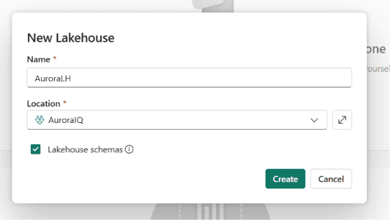
Open AuroraIQ, select + New item, choose Lakehouse, and name it AuroraLH. In the dialog, tick Lakehouse schemas. That checkbox creates the dbo schema, a named folder for tables inside the lakehouse, and every row count at the end of this stage is checked under dbo.
1.2 Upload the files
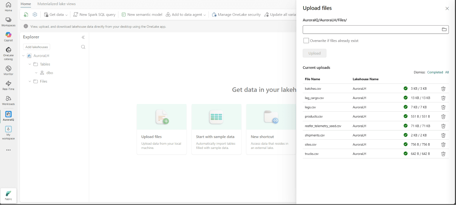
Grab the files first if you have not already: download all eight CSVs from the pharma cold-chain folder of the project files repo, or take the ZIP of all eight in one download.
Upload all eight CSVs to Files. Only six of them become tables:
| File | Becomes a table? | Why |
|---|---|---|
sites.csv | Yes | 12 rows |
products.csv | Yes | 8 rows. Carries each product's safe band and excursion budget. |
trucks.csv | Yes | 12 rows |
shipments.csv | Yes | 33 rows |
batches.csv | Yes | 61 rows |
legs.csv | Yes | 77 rows. The journey itself: one row per leg, and a leg is simply one truck driving from one site to the next. |
leg_cargo.csv | No | Goes to the Eventhouse in Stage 3. |
reefer_telemetry_seed.csv | No | Gets replayed through the Eventstream in Stage 2. |
That last row matters more than it looks. The telemetry never becomes a lakehouse table. It reaches the Eventhouse through the same pipe live data uses, because the point of this build is that there is only one path for sensor data, not a real one and a demo one.
1.3 Load the six tables
Files are just files sitting in storage. Nothing later in this build can query a CSV directly: the ontology you build in Part 2 of this series only reads Delta tables, the lakehouse's table format, which is a real database table with named, typed columns rather than a plain text file. So each CSV needs converting once. There are two ways to do it, below. Pick one, not both. They load the same six tables, so running both overwrites your work and spends capacity twice. Method 1 is the one to use.
Method 1: one notebook cell (recommended)
A notebook is a page in Fabric where you write small pieces of code in cells and run them. The code runs on Spark, the engine Fabric uses for this kind of work, and every run happens inside a Spark session, a temporary claim on your capacity that lasts until it times out. This method writes all six tables in one session, so it never trips the capacity limit the manual clicks can (more on that below).
- In the
AuroraIQworkspace, select + New item, then Notebook. Name itLoad Aurora data. - In the notebook's left Explorer, select Add data items, then From OneLake catalog. Pick the
AuroraLHlakehouse and select Connect. AuroraLHnow shows under Explorer. Hover it, select the pin icon (or its ⋯ menu), and set it as the default lakehouse. This is what the relativeFiles/path in the code resolves against.- Paste this into the first cell and select Run. One Spark session writes all six tables and prints each as it lands:
tables = ["sites", "products", "trucks", "shipments", "batches", "legs"]

for t in tables:
    (spark.read
        .option("header", "true")
        .option("inferSchema", "true")
        .csv(f"Files/{t}.csv")
        .write.mode("overwrite").format("delta")
        .saveAsTable(f"dbo.{t}"))
    print(f"loaded {t}")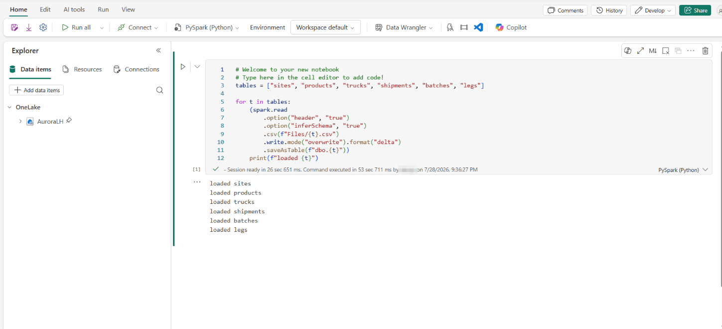
Method 2: load each file by hand
Use this only if you skipped Method 1. In the AuroraLH lakehouse, under Files, right click a CSV, select Load to Tables, then New table.
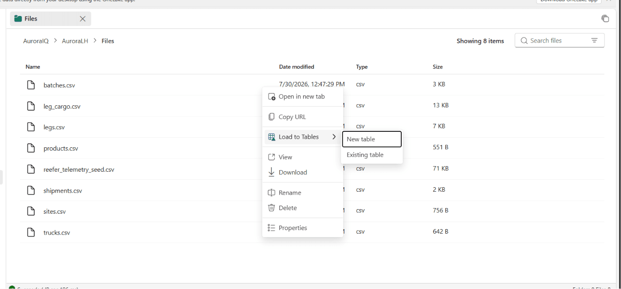
A dialog opens with four fields:
- Keep Schema as
dbo. - Keep the suggested table name.
- Leave Use header for column names ticked.
- Select Load.
Repeat for the six static files only. leg_cargo and reefer_telemetry_seed.csv stay as files, for the reasons in 1.2. Clicking through it once is worth doing the first time, because you see exactly what each step produces. But read the box below before you fire off six in a row.
Whichever method you used, go back to the AuroraLH lakehouse and expand Tables, then dbo. All six should be there. Check the row counts:
| Table | Expected rows |
|---|---|
sites | 12 |
products | 8 |
trucks | 12 |
shipments | 33 |
batches | 61 |
legs | 77 |
Stage 2: give the data a present tense with an Eventstream and an Eventhouse
This is where Real-Time Intelligence comes in, and where this build stops resembling a normal analytics project. Real-Time Intelligence is Fabric's home for data that never stops arriving. Everything you create in this stage, the Eventstream and the Eventhouse, is a Real-Time Intelligence item.
Where you are: the facts are loaded, but nothing moves. This stage builds the live pipe in seven short steps; at the end, twelve trucks report every thirty seconds into a table you can query.
2.1 Create the Eventhouse
In the AuroraIQ workspace: + New item, Eventhouse, named AuroraEH. That is the whole step, but notice what it quietly did for you.
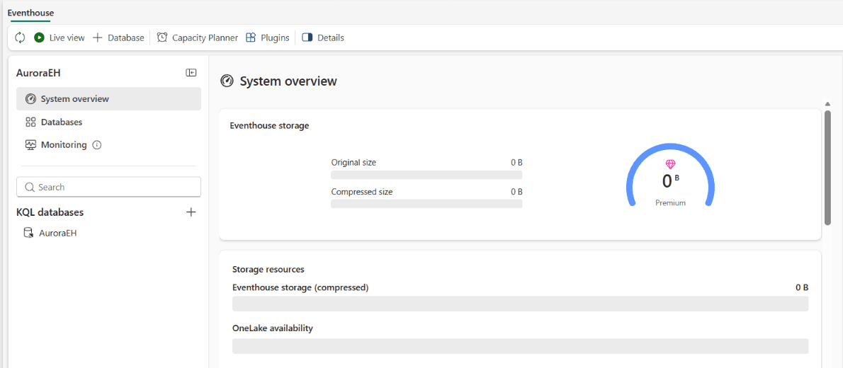
An Eventhouse is the container. The KQL database inside it, listed on the left with the same name, is the thing you actually query and the thing the ontology binds to. Storage reads 0 B because nothing has arrived yet. That number moving is how you will know the pipeline works.
2.2 Create the Eventstream and its custom endpoint
In the AuroraIQ workspace: + New item, Eventstream, named ReeferTelemetryES. Choose Use custom endpoint, or Add source then Custom endpoint if you are already in the editor. A custom endpoint is an address the stream listens on. Anything that can reach that address can push events into the stream. Our notebook will play the part of the trucks in 2.5, so an address is all we need.
The dialog asks for a Source name. The source is the box on the eventstream canvas that stands for whoever sends the events. Here that is the twelve refrigerated trucks (the reefers, from the start of this article), with the notebook playing their part, so name it ReeferTrucks instead of the default CustomEndpoint-Source. The name is only a label, so nothing breaks either way; the right one just makes the canvas read as the story it is: trucks send, the stream carries, the Eventhouse keeps.
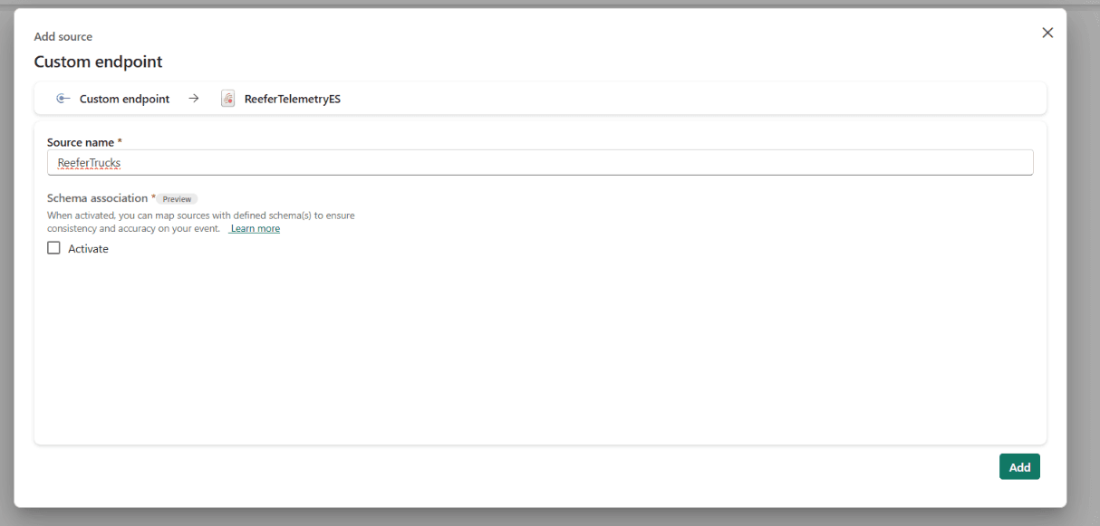
Select Add. The canvas now shows your source feeding the stream, with an empty slot where a destination belongs, and a banner saying changes go live when you publish.
Leave it unpublished for one more step. One publish can cover the source and the destination together.
2.3 Route the stream into the Eventhouse
There are two ways to add a destination, and one of them saves you a small fight.
On the canvas, the stream node has an empty card next to it reading Transform events or add destination. Click that. Adding a destination this way arrives already wired to the stream.
The ribbon's Add destination button does the same job but drops the node onto the canvas unconnected, and you draw the link yourself afterwards. Both end up in the same place. The card is fewer steps.
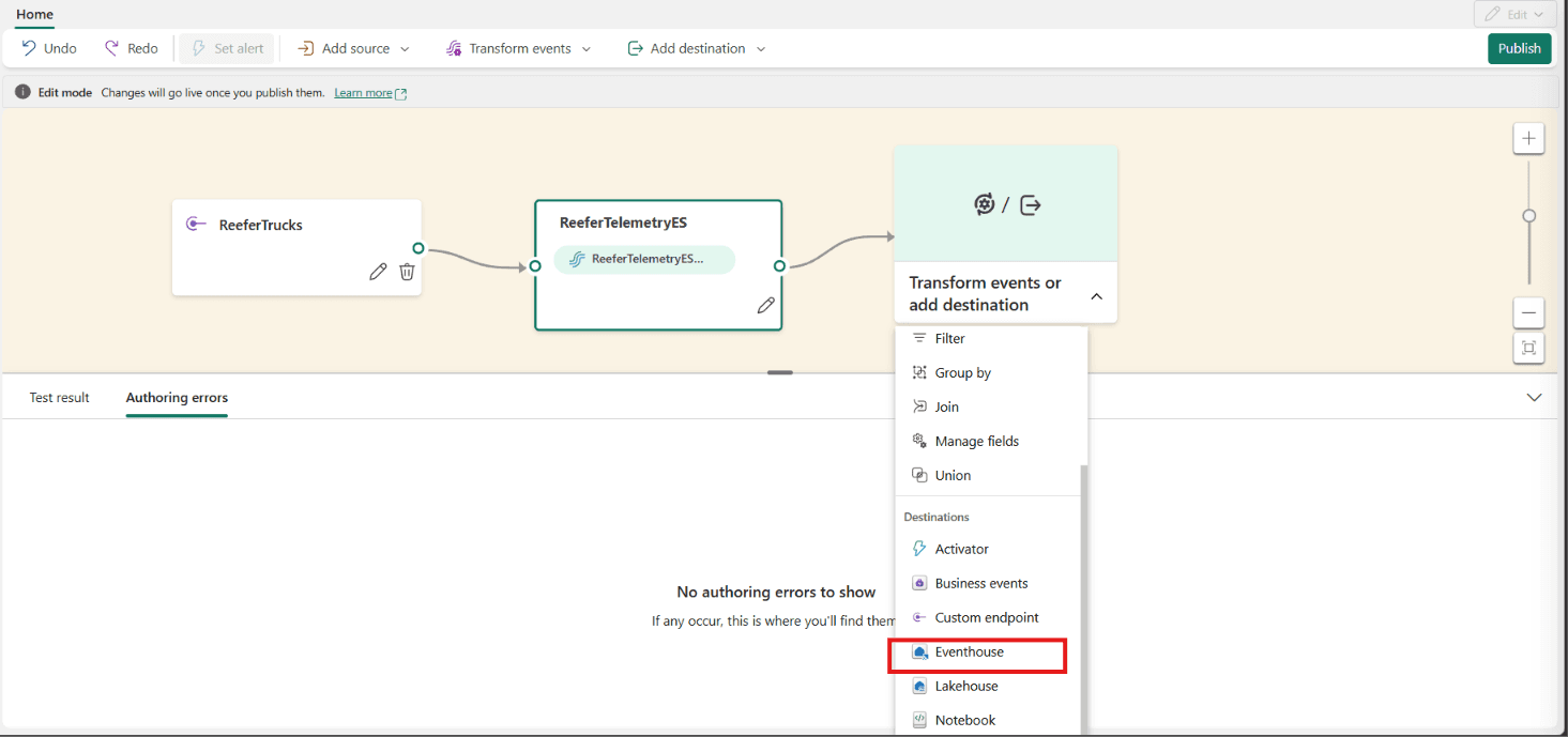
The menu leads with what you can do to the events. Filter, Group by, Join, Manage fields and Union come first, and the Destinations group sits below them. Scroll past the transforms and choose Eventhouse.
A panel opens on the right. The first choice on it is Data ingestion mode, and it offers two options. Ingestion is simply the word for data being written into a database, and the mode controls whether events are changed on the way in. Direct ingestion means events land in the table exactly as they arrive, which is what we want, because all the enrichment happens later in KQL where it can be inspected and corrected. The alternative, Event processing before ingestion, transforms events in the stream instead.
So fill in the panel:
| Panel field | Set it to |
|---|---|
| Data ingestion mode | Direct ingestion |
| Destination name | Leave the default, Eventhouse |
| Workspace | AuroraIQ |
| Eventhouse | AuroraEH |
| KQL Database | AuroraEH |
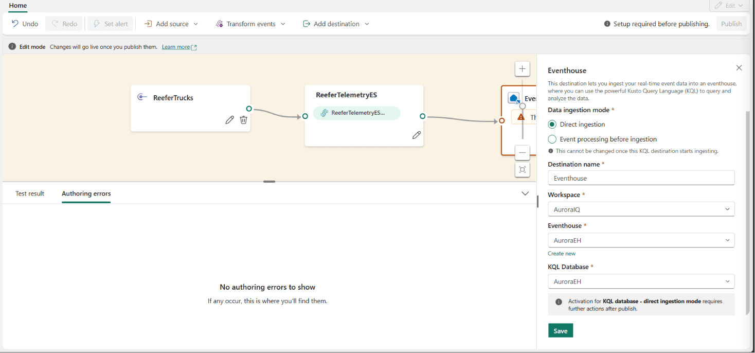
Notice what the panel never asks for: a table name. That is not an oversight. The grey note at the bottom says "Activation for KQL database - direct ingestion mode requires further actions after publish." In other words, Fabric is telling you the table gets chosen later, in a separate step, which is exactly why the next two sections look the way they do.
Select Save.
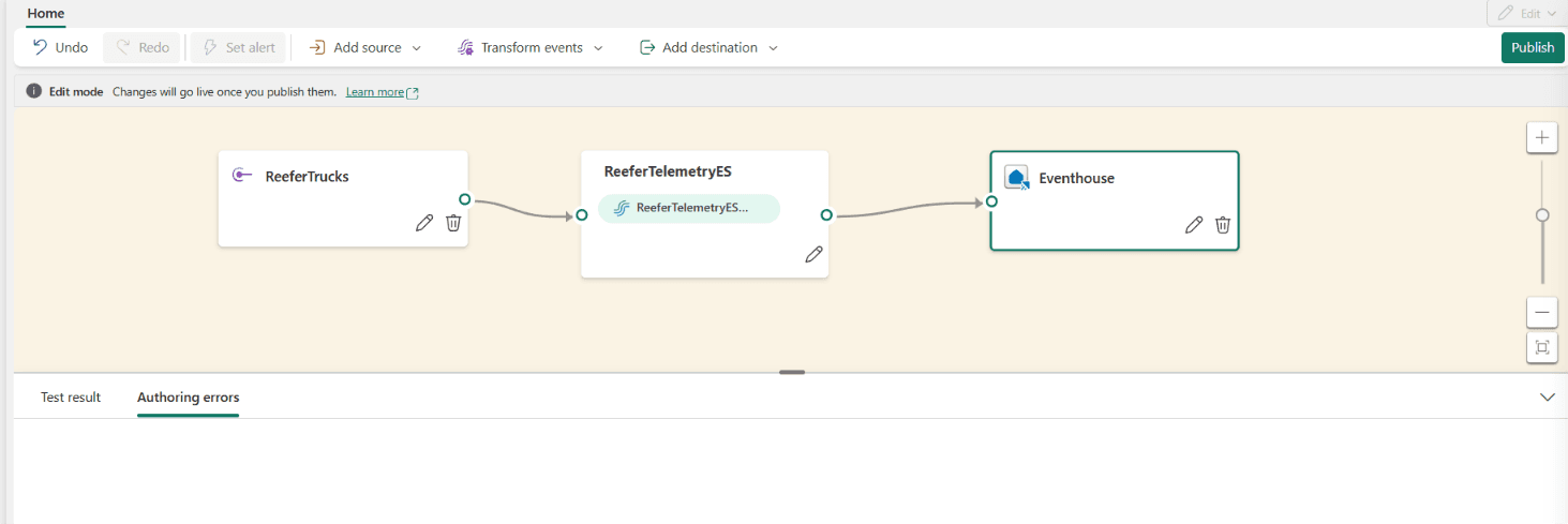
Check that Authoring errors is empty, then select Publish.
That is the whole ingestion path. A truck anywhere with a network connection sends to the first box, and the reading lands in a queryable database seconds later, with nothing scheduled and no file exported by anyone.
2.4 Collect the connection details
Publishing did two things. It created the Live view, which is where the connection details live, and it changed how the canvas reads.
Look at the three nodes now. Each one is in a different state, and all three are correct:
| On the canvas | It reads | Why that is right |
|---|---|---|
ReeferTrucks, the source | Active | It is live and listening. |
| The Eventhouse destination | Unconfigured, with a Configure button | It is waiting for a table, the "further actions after publish" the panel warned about. |
| The data preview | No data to preview | Nothing has sent an event yet. |
The next three steps fix them in that order.
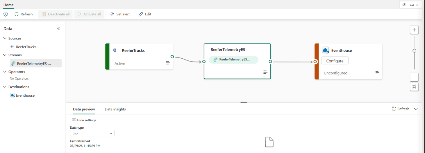
The left panel is a useful summary of what an eventstream is: Sources, Streams, Operators, Destinations. Ours has one of each and no operators, because we deliberately do no transformation in the stream. Every reading lands exactly as the truck sent it, and all the interpretation happens afterwards in KQL where you can read it, test it, and fix it.
Select the ReeferTrucks node and open its Details pane. There are three protocol tabs: Event Hub, AMQP, and Kafka.
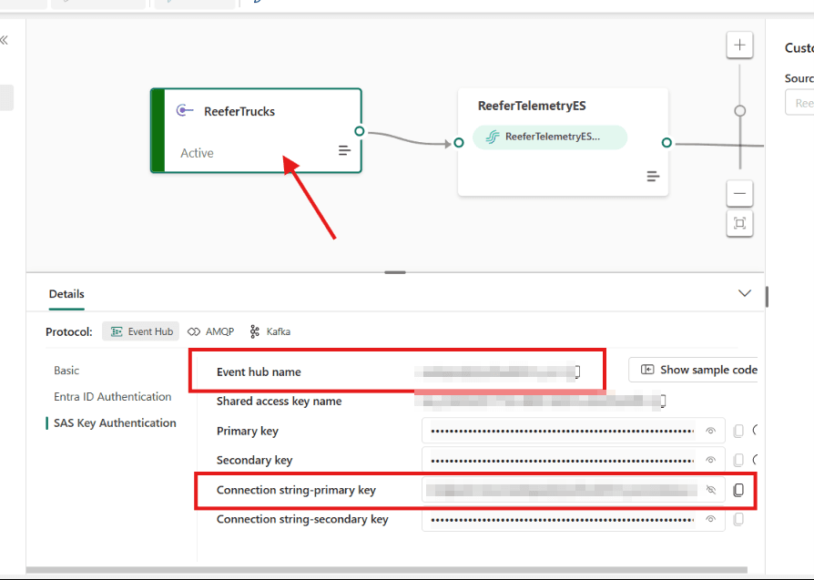
This pane is worth pausing on. An Eventstream custom endpoint speaks the Event Hubs protocol, which means anything that can talk to Azure Event Hubs can talk to Fabric without knowing Fabric exists. Your fleet does not need a Fabric SDK. It needs an address.
Stay on the Event Hub tab. Its SAS Key Authentication section holds the two values you need. SAS is short for shared access signature: a password-like key that lets a sender write to this endpoint. Take both values using the copy icon beside each:
| Copy this field | Where it goes, in 2.5 |
|---|---|
| Connection string-primary key | The CONNECTION_STRING placeholder in the connect cell |
| Event hub name | The EVENT_HUB_NAME placeholder in the connect cell |
Treat the connection string as a password. It carries write access to your eventstream, so anything holding it can push events into your pipeline. The primary and secondary keys exist so you can rotate one while the other keeps working.
2.5 Send five events before you create the table
This step looks out of order and is not.
The Configure button on the destination node is the next thing the interface offers, and it is tempting. Leave it alone for a few more minutes.
The Eventhouse Get data wizard never asks which columns you want. It builds the table by looking at events that have already travelled through the stream, and copies their shape. It sees TempC holding numbers, so it makes a number column. It sees TruckID holding text, so it makes a text column. Working the columns out from real data like this is called schema inference.
Your stream has carried nothing so far. So the wizard has nothing to copy, and you finish with an empty or wrong set of columns. Nothing warns you. You find out much later, when a query returns nothing and there is no obvious reason why.
So put five events into the stream first, and let the wizard copy those. Five throwaway readings from one truck is enough. A tiny run like this, done only to prove the pipe works at all, is called a smoke test, which is why the code below names the list smoke.
Two setup steps first:
- In the
AuroraIQworkspace, select + New item, then Notebook. Name itSend reefer telemetry. The rest of this article calls it the sender notebook. - In the notebook's left Explorer, attach the
AuroraLHlakehouse and pin it as the default, exactly as you did in 1.3. The cells below do not need it, but the backfill in 2.7 reads CSVs fromFiles/, so doing it now saves a trip back.
Then three cells, each in its own cell of the notebook. Add each with + Code, run it, and check its output before you add the next one.
Cell 1 — the install
Paste this into the first cell and select Run. Fabric's default Python image does not carry the library that speaks the Event Hubs protocol, so install it before anything imports it. Takes about twenty seconds:
%pip install azure-eventhubKeep it in a cell of its own at the top of the notebook. Fabric expects %pip install at the start, and sharing a cell with the imports means every re-run pays the install again.
The install belongs to the notebook session, not to the notebook. When Fabric ends an idle session, the library goes with it, so coming back on another day means running this cell again before the connect cell.
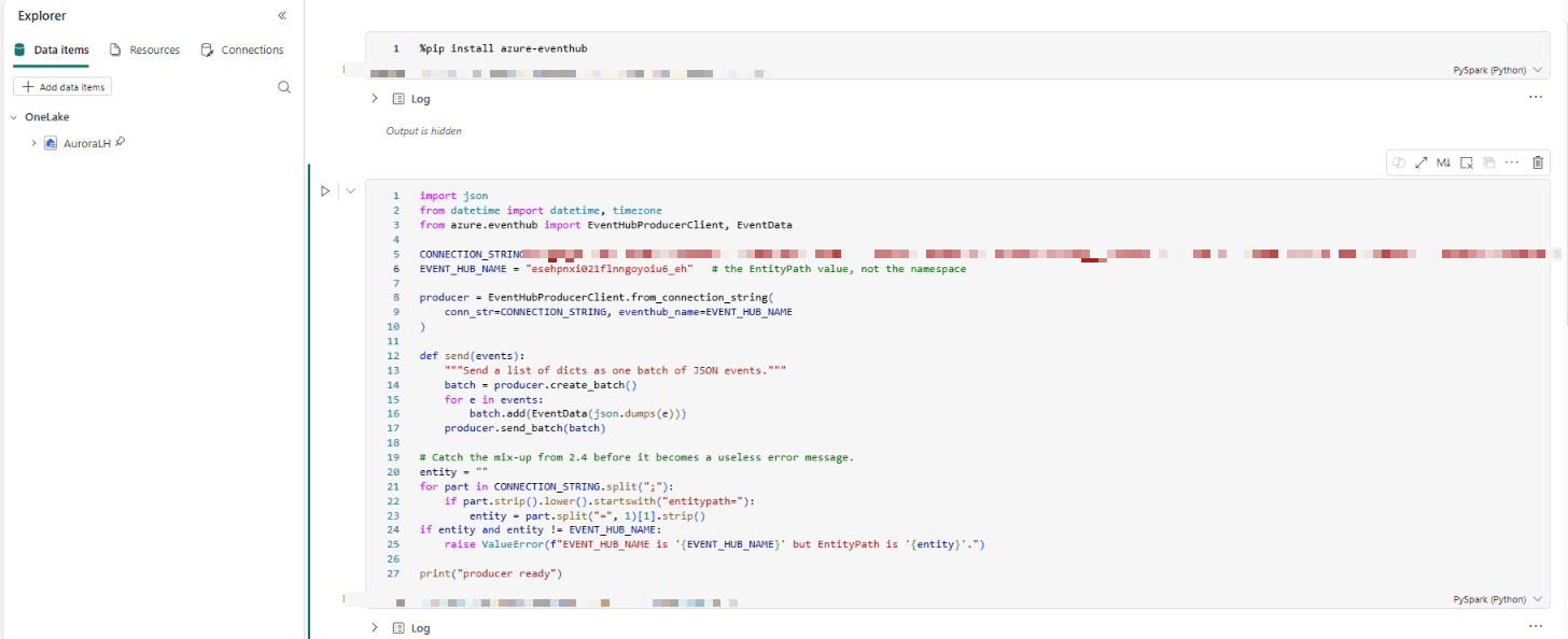
Cell 2 — the connect cell
Paste this into a second cell. Replace the two placeholder strings with the Connection string-primary key and Event hub name you copied in 2.4, then select Run:
import json
from datetime import datetime, timezone
from azure.eventhub import EventHubProducerClient, EventData

CONNECTION_STRING = "PASTE-CONNECTION-STRING-PRIMARY-KEY-HERE"
EVENT_HUB_NAME = "PASTE-EVENT-HUB-NAME-HERE"   # the EntityPath value, not the namespace

producer = EventHubProducerClient.from_connection_string(
    conn_str=CONNECTION_STRING, eventhub_name=EVENT_HUB_NAME
)

def send(events):
    """Send a list of dicts as one batch of JSON events."""
    batch = producer.create_batch()
    for e in events:
        batch.add(EventData(json.dumps(e)))
    producer.send_batch(batch)

# Catch the mix-up from 2.4 before it becomes a useless error message.
entity = ""
for part in CONNECTION_STRING.split(";"):
    if part.strip().lower().startswith("entitypath="):
        entity = part.split("=", 1)[1].strip()
if entity and entity != EVENT_HUB_NAME:
    raise ValueError(f"EVENT_HUB_NAME is '{EVENT_HUB_NAME}' but EntityPath is '{entity}'.")

print("producer ready")
This cell reads no files on purpose. If it fails, the problem is the credential and nothing else, and you have not wasted time wondering whether a CSV was missing.
Cell 3 — the smoke test
Paste this into a third cell and select Run. It sends five readings from one truck, two seconds of work:
smoke = [
    {
        "TruckID": "TRK-01",
        "Timestamp": datetime.now(timezone.utc).strftime("%Y-%m-%dT%H:%M:%SZ"),
        "TempC": round(4.6 + i * 0.1, 1),
        "HumidityPct": 44 + i,
        "IntervalMinutes": 15.0,
    }
    for i in range(5)
]
send(smoke)
print("sent 5 events, fields:", sorted(smoke[0].keys()))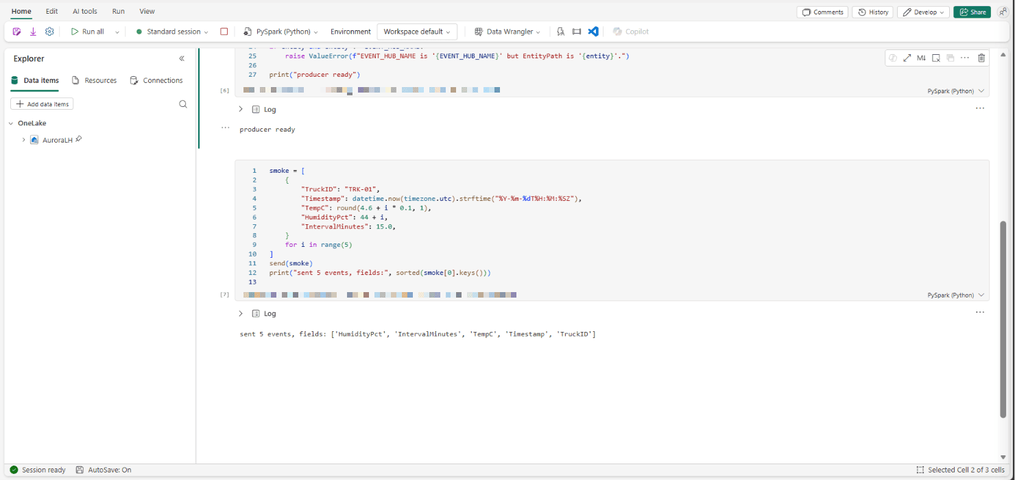
Now go back to the ReeferTelemetryES eventstream and open the Live view. Select Refresh on the data preview at the bottom. Five rows appear, and No data to preview is gone. That is the wizard's raw material.
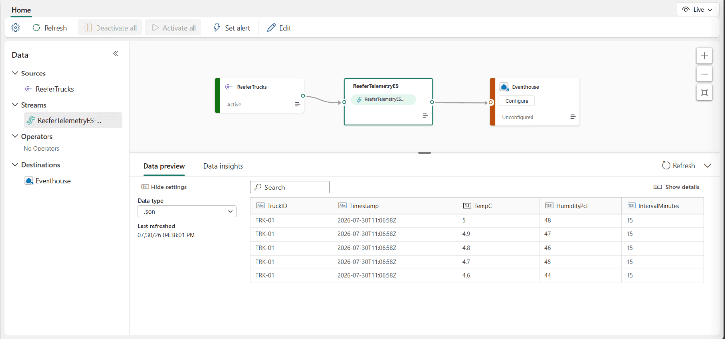
2.6 Create the table
Now select Configure on the destination node, the button that has been waiting since you published. The Eventhouse Get data wizard opens. It runs in four steps, listed down the left: Source, Configure, Inspect, Summary.
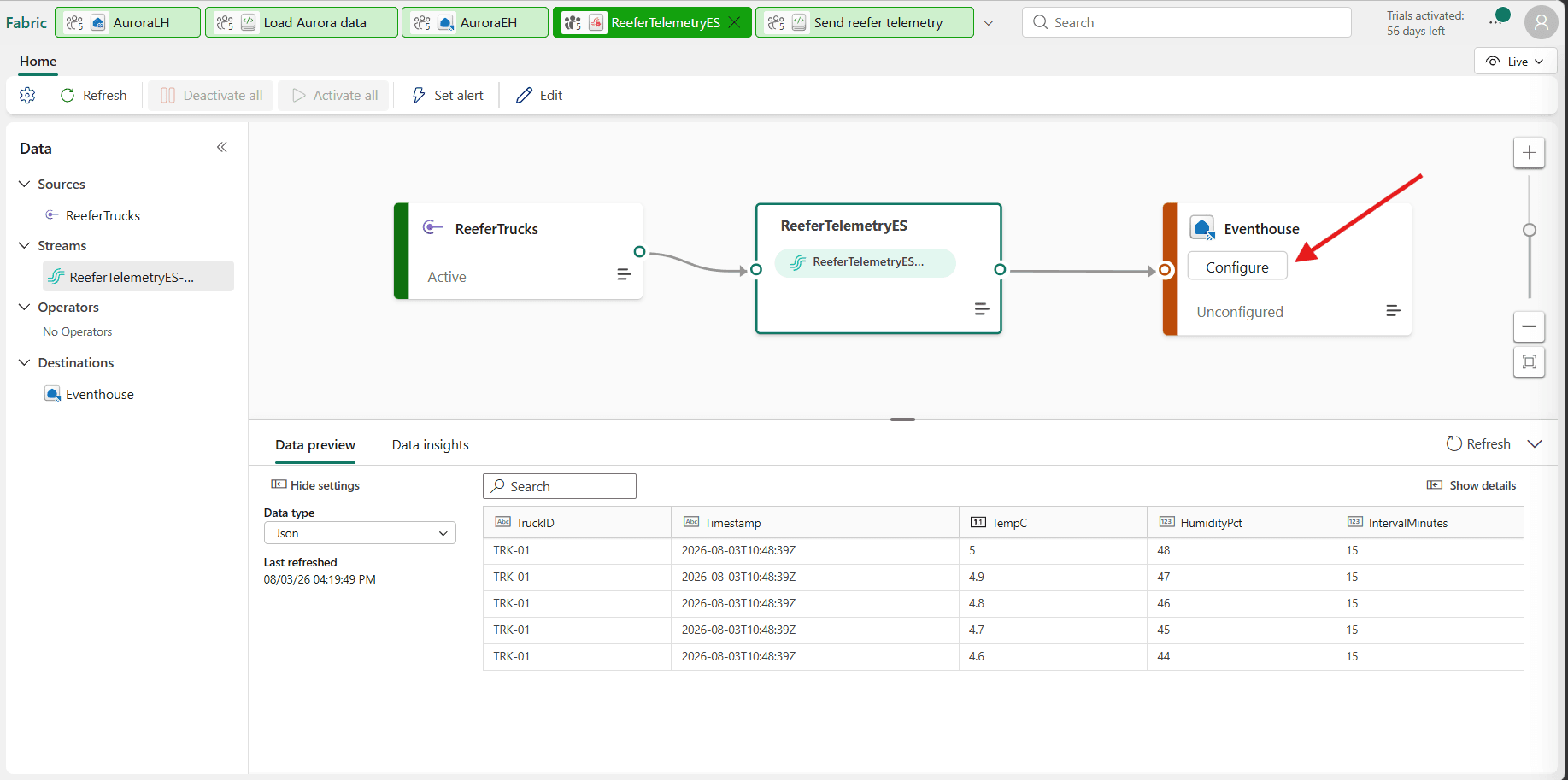
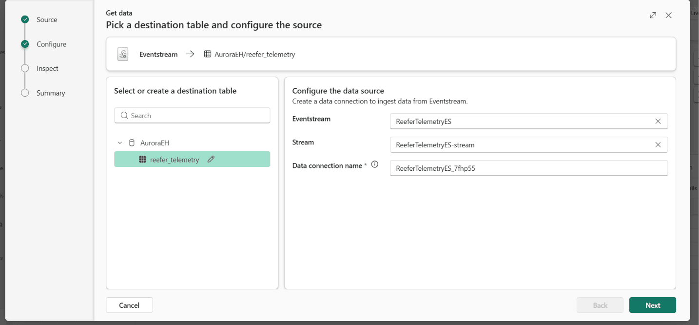
Source. Choose New table and name it reefer_telemetry. This is the destination table: it lives inside the AuroraEH KQL database, and from the moment this wizard finishes, every reading the stream carries lands in it as one row.
Configure. Your new table appears under the AuroraEH KQL database on the left, already selected. The right side fills itself in: Eventstream is ReeferTelemetryES, Stream is ReeferTelemetryES-stream, and Data connection name carries a generated value like ReeferTelemetryES_7fhp55.
Leave the connection name alone. It names an internal connection object, nothing else in this build refers to it, and the random suffix is there to keep it unique. Select Next.
Inspect. This is the payoff for the previous section. The wizard shows your five events and infers five columns from them. Set the format to JSON, then check the type it chose for each column before you finish.
Select the ✏️ beside the mapping name to open the column editor. Each column gets a row with its Type in a dropdown you can change. This is what the five rows should read before you press Apply:
| Column | Correct type | What the wizard infers |
|---|---|---|
TruckID | string | string, correct on its own |
Timestamp | datetime | datetime, correct on its own |
TempC | real | real, correct on its own |
HumidityPct | int | int, correct on its own |
IntervalMinutes | real | int — wrong, change it by hand |
Only IntervalMinutes needs your hand, for the reason in the callout above: the smoke events all carried 15.0, so the wizard saw whole numbers. The other four come through right; confirm them rather than trusting them.
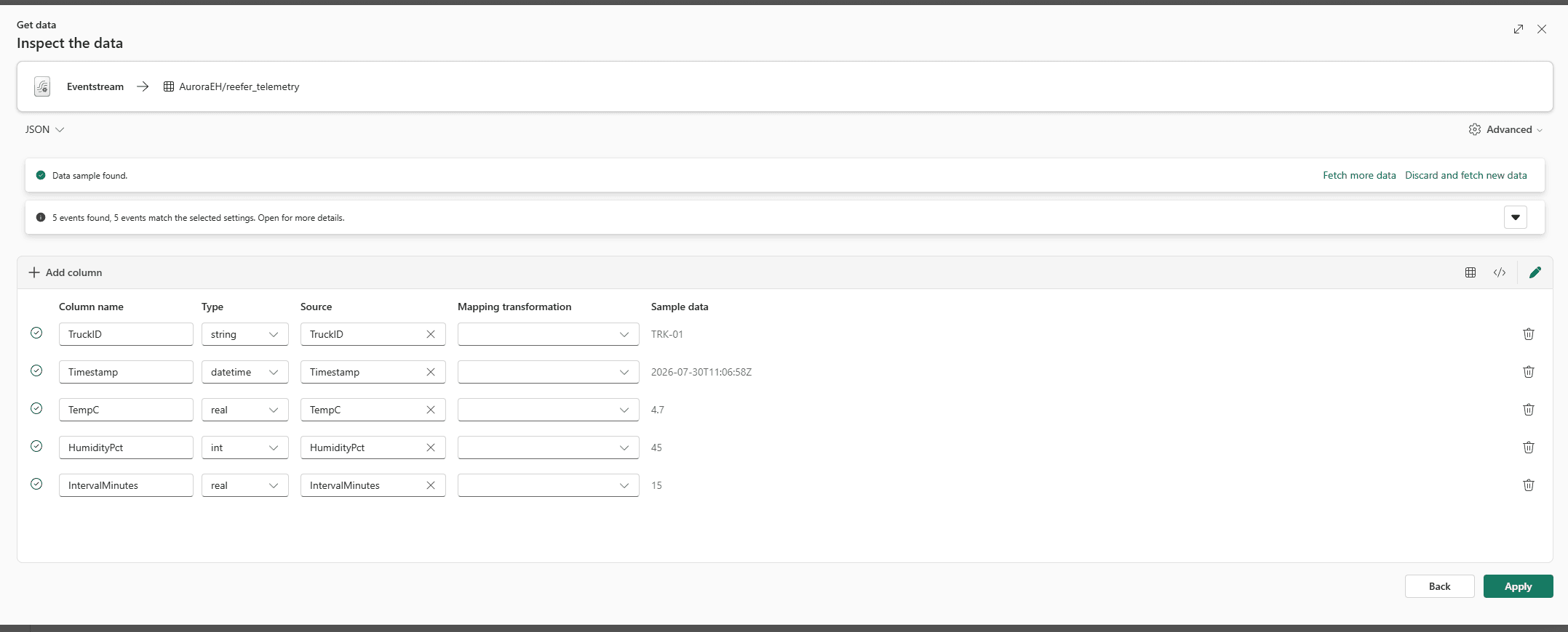
Select Apply. That is the commit point for the column types, so read the list once more first. Everything above that button is still editable, and nothing below it is.
Summary. The last step lists the three things it built:
| It built | In this build | What it does |
|---|---|---|
| A table | reefer_telemetry | Every reading the stream carries lands in it as one row. |
| A mapping | reefer_telemetry_mapping | Holds the column types you set on the Inspect step. |
| A data connection | The generated name from the Configure step | Moves events from the stream into the table. |
Select Close, and the destination node on the canvas stops saying Unconfigured.
The page also offers Delete ingested data under "Undo ingestion". Ignore it, and do not be surprised when the table turns out to be empty. Query it now and you get no rows at all.
That is correct. Your five smoke events were sent before this table existed, which was their entire purpose. The wizard read them to work out the columns, but the data connection you just created only starts consuming from the moment it is created, so those five events were never ingested. They shaped the table without ever entering it.
Nothing in reefer_telemetry until 2.7 sends something new.
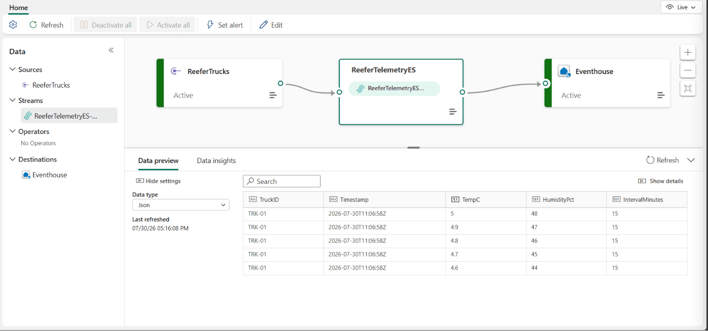
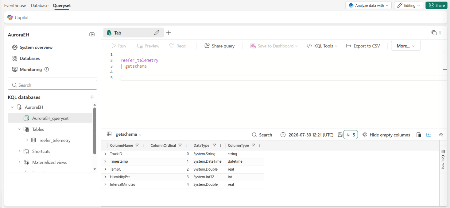
That is the pipe built, configured and proved. But the table is still empty: the only traffic so far was five hand-sent readings that shaped the columns without ever entering it. Everything the rest of this article depends on still has to arrive.
2.7 Simulate the trucks and fill the table
The table exists and the pipe works. Now fill it.
Two things go in, in this order. The backfill replays the recorded journeys, so the Eventhouse holds history the moment the ontology binds to it in Stage 4. The live stream then keeps twelve trucks reporting until you stop it.
Both run from the sender notebook you built in 2.5. Open the Send reefer telemetry notebook from the AuroraIQ workspace; everything in this section happens in it, reusing the send() function already defined there.
It already holds three cells: cell 1, the %pip install; cell 2, the connect cell; and cell 3, the smoke test. This section adds four more. Add each with + Code, run it, and check its output before you add the next one. They depend on each other in order.
| Cell | Does | Prints |
|---|---|---|
| 1–3 | already built in 2.5 | |
| 4 | defines the fleet | 12 trucks ready |
| 5 | replays the recorded journeys | 400/1812 … backfill complete |
| 6 | shifts the leg files to match | wrote shifted_legs.csv … |
| 7 | streams live, until you stop it | sent 12 events, repeating |
One numbering note: this article counts cells by their position in the notebook, top to bottom. The bracket on a cell's left edge, like [9], is the session's execution counter — it climbs with every run and re-run, so it will not match the position numbers here. When a step says "cell 7", count from the top.
Cell 4 — the fleet
Paste this into a new cell and Run. It builds the fleet and sends nothing. Nothing reaches Fabric until cell 5:
import random
import time
from datetime import datetime, timezone, timedelta
import pandas as pd

FILES = "/lakehouse/default/Files"
SEND_EVERY_SECONDS = 30          # live pacing, denser than the 15-minute seed

# The live incident, used in Stage 5 (Part 2 of the series). TRK-04's reefer fails.
INCIDENT_TRUCK = "TRK-04"
INCIDENT_PEAK_C = 15.5
INCIDENT_RAMP_MIN, INCIDENT_HOLD_MIN, INCIDENT_RECOVER_MIN = 6, 20, 8

legs = pd.read_csv(f"{FILES}/legs.csv")
cargo = pd.read_csv(f"{FILES}/leg_cargo.csv")
trucks = sorted(legs["TruckID"].unique().tolist())

# Each truck's target is the midpoint of the safe band of what it carries.
band = cargo.groupby("TruckID")[["MinSafeC", "MaxSafeC"]].mean()
SETPOINT = {
    t: float((band.loc[t, "MinSafeC"] + band.loc[t, "MaxSafeC"]) / 2) if t in band.index else 5.0
    for t in trucks
}
_state = {t: {"temp": SETPOINT[t], "hum": random.randint(38, 52)} for t in trucks}


def _incident_temp(elapsed_s, start_s):
    """Ramp, hold, recover profile for the incident truck. None otherwise."""
    if start_s is None:
        return None
    t_min = (elapsed_s - start_s) / 60
    if t_min < 0:
        return None
    base = SETPOINT[INCIDENT_TRUCK]
    if t_min < INCIDENT_RAMP_MIN:
        return base + (INCIDENT_PEAK_C - base) * (t_min / INCIDENT_RAMP_MIN)
    if t_min < INCIDENT_RAMP_MIN + INCIDENT_HOLD_MIN:
        return INCIDENT_PEAK_C
    t_rec = t_min - INCIDENT_RAMP_MIN - INCIDENT_HOLD_MIN
    if t_rec < INCIDENT_RECOVER_MIN:
        return INCIDENT_PEAK_C + (base - INCIDENT_PEAK_C) * (t_rec / INCIDENT_RECOVER_MIN)
    return None


def _reading(truck_id, forced=None):
    s, base = _state[truck_id], SETPOINT[truck_id]
    if forced is not None:
        s["temp"] = forced + random.uniform(-0.2, 0.2)
        s["hum"] = min(80, s["hum"] + random.randint(0, 2))
    elif random.random() < 0.04:
        # A door opening at a dock. Warm air gets in, so the temperature always
        # goes UP: a chilled truck to about 13.9C, a frozen one to about -6.5C.
        # Both break their own ceiling, which is what a door opening really is.
        s["temp"] = base + (8.9 if base > 0 else 13.5) + random.uniform(-0.6, 0.6)
        s["hum"] = min(78, s["hum"] + random.randint(6, 11))
    else:
        s["temp"] += 0.4 * (base - s["temp"]) + random.uniform(-0.2, 0.2)
        s["hum"] = round(s["hum"] + 0.35 * (random.randint(38, 52) - s["hum"]) + random.uniform(-1.2, 1.2))
    return {
        "TruckID": truck_id,
        "Timestamp": datetime.now(timezone.utc).strftime("%Y-%m-%dT%H:%M:%SZ"),
        "TempC": round(s["temp"], 1),
        "HumidityPct": int(max(30, min(80, s["hum"]))),
        "IntervalMinutes": round(SEND_EVERY_SECONDS / 60.0, 3),
    }


def run_stream(incident=False, incident_after_min=2):
    """Stream readings until interrupted. State carries across calls."""
    t0, sent = time.time(), 0
    start_s = incident_after_min * 60 if incident else None
    print(f"streaming, one reading per truck every {SEND_EVERY_SECONDS}s. Interrupt to stop.")
    while True:
        forced = _incident_temp(time.time() - t0, start_s)
        send([_reading(t, forced if t == INCIDENT_TRUCK else None) for t in trucks])
        sent += len(trucks)
        print(f"sent {sent} events")
        time.sleep(SEND_EVERY_SECONDS)


print(f"{len(trucks)} trucks ready")
Four decisions in there are what make the result believable rather than random:
- Setpoints come from the cargo, not from thin air. Each truck's target is the midpoint of the safe band of whatever it is actually carrying, averaged from
leg_cargo. A truck of insulin sits at 5°C, a truck of frozen vaccine at -20°C. The live stream continues the recorded journeys' physics instead of inventing new ones. - Each reading drifts toward its setpoint.
temp += 0.4 * (setpoint - temp)plus jitter. That is a thermostat closing 40% of the gap each tick. - Four percent of readings are a door opening at a dock. Warm air gets in, so the temperature always goes up, past whichever ceiling that truck has. This is deliberate. It is the innocent noise that defeats the naive "alert above 8°C" rule from the start of this article, and without it the demo would be too clean to prove anything.
IntervalMinutesis declared per reading. The recorded journeys say15.0, live readings say0.5. The KQL in Stage 3 reads the field rather than assuming a cadence, so one piece of code scores both correctly. Hardcode either value and you silently multiply every exposure figure for the other.
Cell 5 — the backfill
Run this once:
SHIFT_TO_NOW = True

seed = pd.read_csv(f"{FILES}/reefer_telemetry_seed.csv")
seed["Timestamp"] = pd.to_datetime(seed["Timestamp"], utc=True, format="ISO8601")

offset = timedelta(0)
if SHIFT_TO_NOW:
    offset = datetime.now(timezone.utc) - seed["Timestamp"].max().to_pydatetime()
    print(f"shifting the recording forward by {offset}")

rows = seed.to_dict("records")
BATCH = 400
for i in range(0, len(rows), BATCH):
    send([
        {
            "TruckID": r["TruckID"],
            "Timestamp": (r["Timestamp"].to_pydatetime() + offset).strftime("%Y-%m-%dT%H:%M:%SZ"),
            "TempC": float(r["TempC"]),
            "HumidityPct": int(r["HumidityPct"]),
            "IntervalMinutes": float(r["IntervalMinutes"]),
        }
        for r in rows[i : i + BATCH]
    ])
    print(f"  {min(i + BATCH, len(rows))}/{len(rows)}")
print("backfill complete")
If it stops with NameError: name 'send' is not defined, cell 2, the connect cell, has not run in this session. Run cell 2, then run this cell again.
Cell 6 — shift the leg files to match
Only needed if you left SHIFT_TO_NOW = True, which you almost certainly did. It must run in the same session as cell 5, because it reuses that cell's offset variable.
It writes shifted_legs.csv and shifted_leg_cargo.csv beside the originals in Files/. There is nothing to upload right now. From here on, whenever a step asks for legs.csv or leg_cargo.csv, use the shifted_ copy instead. Section 3.2 covers both: it loads shifted_leg_cargo.csv into the Eventhouse and reloads the legs table from 1.3, which keeps its old dates until then:
if SHIFT_TO_NOW:
    for name in ("legs.csv", "leg_cargo.csv"):
        df = pd.read_csv(f"{FILES}/{name}")
        for col in ("DepartUtc", "ArriveUtc"):
            df[col] = (pd.to_datetime(df[col], utc=True, format="ISO8601") + offset).dt.strftime("%Y-%m-%dT%H:%M:%SZ")
        df.to_csv(f"{FILES}/shifted_{name}", index=False)
        print(f"wrote shifted_{name}")
Cell 7 — the live stream
One line. It runs until you interrupt it, so leave it going while you build the rest of the article:
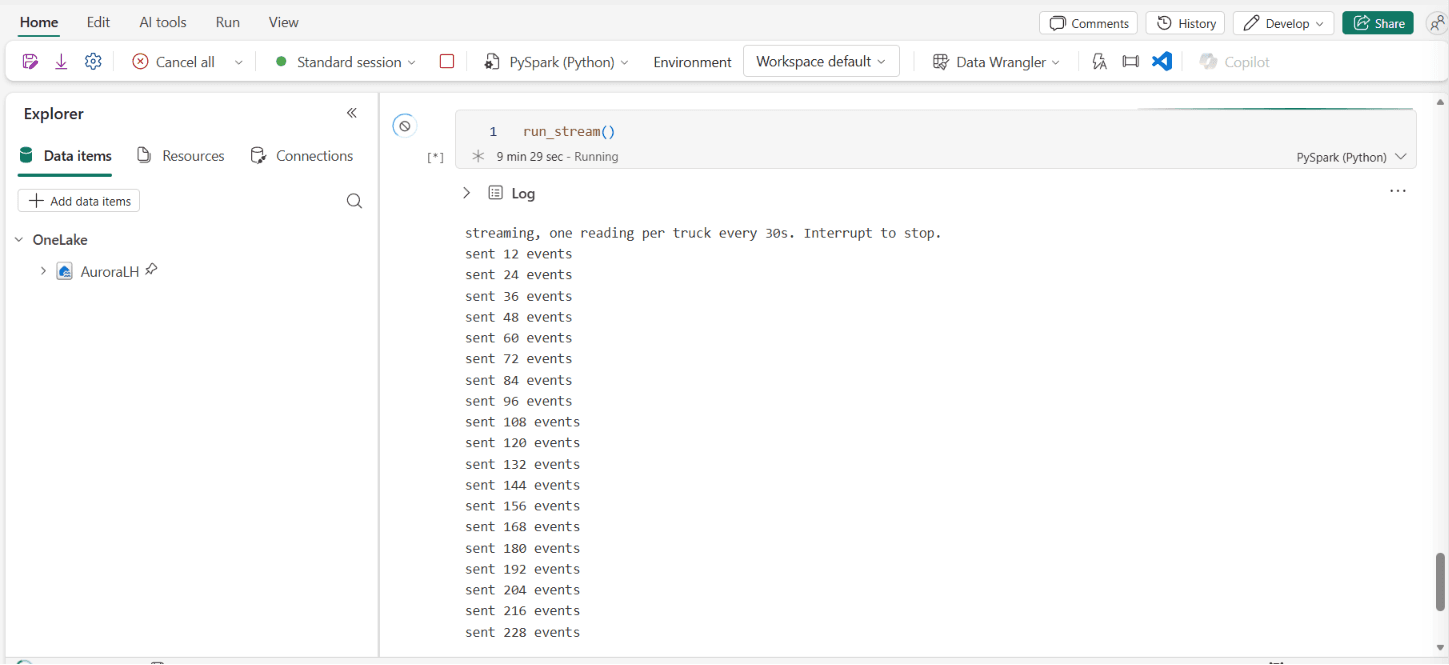
run_stream()It prints sent 12 events, then sent 24 events, and so on every thirty seconds. The cell stays marked [*] and running, which is correct. Do not wait for it to finish, because it never will. Use the stop button when you want it to end, and re-run it to start again.
Confirm data is landing
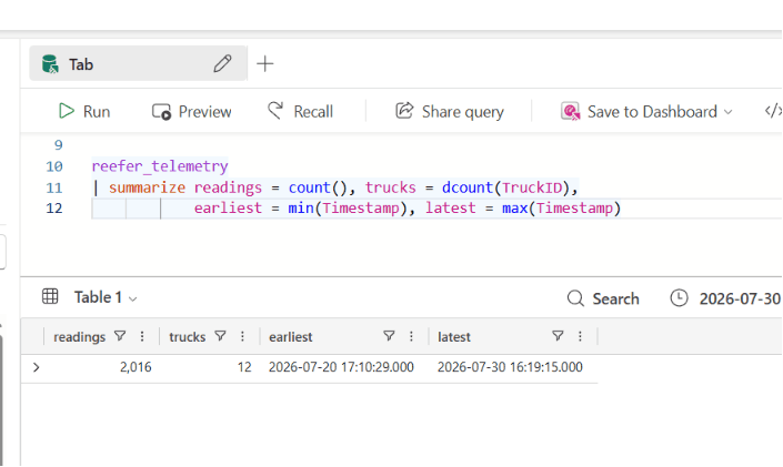
This last check is not a notebook cell. It is KQL, and it belongs in the Eventhouse.
Back in AuroraEH_queryset, the same editor you ran getschema in (open the AuroraEH Eventhouse and select it in the left tree), run this there:
reefer_telemetry
| summarize readings = count(), trucks = dcount(TruckID),
            earliest = min(Timestamp), latest = max(Timestamp)
Give it a minute or two first. Eventhouse batches ingestion, so data sent seconds ago is not queryable yet, and an empty result right after cell 5 means nothing.
What you want back:
| Column | Expect | What it tells you |
|---|---|---|
readings | 1,812 and climbing | the backfill landed, and cell 7 is adding twelve every thirty seconds |
trucks | 12 | the whole fleet reported, not just one |
latest | within minutes of now | SHIFT_TO_NOW worked, so the recording ends today rather than last week |
earliest | about ten days before latest | the journeys kept their relative spacing through the shift |
latest is the one to read carefully. If it sits days in the past, the shift did not apply, and Stage 3 will join nothing.
The five smoke events from 2.5 are not in this count and never were, for the reason at the end of 2.6.
What you just did
There are no real trucks. The notebook simulated the whole fleet: the backfill replayed ten days of recorded journeys, and cell 7 keeps twelve pretend trucks reporting every thirty seconds until you stop it. Everything after the notebook, though, is real. The readings travel the same custom endpoint, the same eventstream, and land in the same reefer_telemetry table that readings from real sensors would use. As far as Fabric knows, a fleet is on the road right now, and every stage from here treats it that way.
Stage 3: make the data smart with KQL so the rules can be simple
Everything so far has been plumbing. This stage is the engineering.
A reading arrives saying TRK-10 was 4.2°C at 22:32; it is the row boxed in red below. To know whether that matters, you need to know what TRK-10 was carrying at 22:32, and what the safe range is for that particular product. 4.2°C is exactly right for a truck of insulin and hopelessly warm for a truck of the frozen vaccine. The truck knows neither what it carries nor what that cargo can survive.
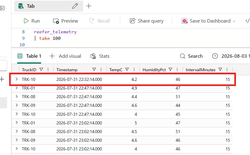
So we join it at the moment it lands.
Six steps, and each one turns the data into something a little more useful than what went in:
| Step | Turns | Into |
|---|---|---|
| 3.1 | nothing | four empty tables with the exact shapes we want |
| 3.2 | a CSV | the shipment plan: who was carrying what, when |
| 3.3 | a bare reading | a reading that knows its batch, and whether it broke that batch's limits |
| 3.4 | thousands of scored readings | one running total per batch, kept fresh by the engine |
| 3.5 | that running total | a plain table the operations agent is allowed to read |
| 3.6 | all of it | proof that the numbers are right |
Everything below runs in the same KQL queryset. Open the AuroraEH Eventhouse and select AuroraEH_queryset in the left tree, the same place you ran getschema in 2.6.
3.1 Create the four tables
Why first: you have already been bitten once by letting Fabric guess. In 2.6 the wizard decided IntervalMinutes was a whole number, because every sample it looked at happened to be 15.0, and you had to catch it by hand before pressing Apply.
Declaring the tables up front removes the guessing. The table exists with exactly the types you chose, and the loader in 3.2 fills a table that already knows what it is instead of inventing one from whatever the first few rows look like.
Four tables carry this stage:
| Table | Holds | Made by |
|---|---|---|
reefer_telemetry | the raw readings, one row per truck per interval | already exists, from 2.6 |
leg_cargo | the cargo list for every leg, like a passenger list for every flight: which batches were aboard which truck, between which times | this step |
excursion_events | one row per reading per batch, scored against that batch's own safe band | this step |
batch_exposure | the running total per batch, which the operations agent watches in Stage 6 (Part 2 of this series) | this step |
The script below does three jobs in one go:
| Job | Commands | In this build |
|---|---|---|
| Create the tables | .create table × 4 | all four tables, with the exact column types we chose |
| Describe the columns | .alter-merge ... column-docstrings × 2 | excursion_events and batch_exposure |
| Set retention | .alter-merge ... policy retention × 3 | 90 days for reefer_telemetry and excursion_events, 30 for batch_exposure |
The descriptions are not decoration — Microsoft's own operations agent guidance asks for them: "If a column's purpose is unclear from its name, add a plain-language description by using the description field in your KQL table schema. This description helps the agent interpret data values correctly." The agent in Stage 6 reads these to work out what your columns mean.
Retention is how long each table keeps rows before deleting them automatically. The raw readings stay longest, because a pharmaceutical audit wants the original trace, and 3.6 reconciles against them.
A word on the folder names in the script below. Bronze, Silver, Gold is a common data warehouse naming habit called the medallion pattern, and each of this stage's four tables has a place in it:
| Folder | What lives there | In this build |
|---|---|---|
00-Dimension | Reference data that describes things, rather than recording events | leg_cargo, the shipment plan |
01-Bronze | Data exactly as it arrived | reefer_telemetry, the raw readings |
02-Silver | The same data, cleaned and joined | excursion_events, every reading scored per batch |
03-Gold | The finished numbers people act on | batch_exposure, the running total per batch |
The leading numbers just force the sort order in the tree. The folders are visual grouping only; they change nothing about how a table behaves.
You could run these as nine separate commands. Kusto, the database engine inside your Eventhouse (KQL is short for Kusto Query Language), has a wrapper that runs them as one: .execute database script takes a list of management commands and executes them top to bottom in a single Run.
.execute database script <|
// ---- the four tables --------------------------------------------------
.create table reefer_telemetry (
    TruckID: string, Timestamp: datetime, TempC: real,
    HumidityPct: int, IntervalMinutes: real
) with (folder = "01-Bronze", docstring = "Raw reefer telemetry landed by an Eventstream custom endpoint. One row per truck per reporting interval.")
.create table leg_cargo (
    LegID: string, ShipmentID: string, TruckID: string, BatchID: string,
    ProductID: string, MinSafeC: real, MaxSafeC: real, BudgetMinutes: int,
    DepartUtc: datetime, ArriveUtc: datetime
) with (folder = "00-Dimension", docstring = "Shipment plan. One row per leg per drug batch, carrying that product's safe band and excursion budget.")
.create table excursion_events (
    BatchID: string, LegID: string, TruckID: string, Timestamp: datetime,
    TempC: real, ExcursionMinutes: real, Direction: string,
    BudgetMinutes: int, BudgetPctIncrement: real
) with (folder = "02-Silver", docstring = "One row per telemetry reading per batch riding that truck on that leg. ExcursionMinutes equals the reading interval when the reading is outside the product's safe band, otherwise 0.")
.create table batch_exposure (
    BatchID: string, Timestamp: datetime, CumulativeMinutes: real,
    BudgetMinutes: int, BudgetUsedPct: real, FreezeEventCount: int
) with (folder = "03-Gold", docstring = "Snapshot appended every 5 minutes. Cumulative out-of-range exposure per drug batch across every leg of its journey.")
// ---- plain-language column descriptions, for the agent in Stage 6 -----
.alter-merge table batch_exposure column-docstrings (
    BatchID:           "Unique identifier of a drug batch. Use this to identify the business object.",
    Timestamp:         "UTC time this snapshot was computed by the scheduled aggregation job.",
    CumulativeMinutes: "Total minutes this batch has spent outside its product's safe temperature band, summed across every leg of its journey so far.",
    BudgetMinutes:     "The product's total allowed excursion budget in minutes for the whole journey.",
    BudgetUsedPct:     "CumulativeMinutes as a percentage of BudgetMinutes. 100 means the batch has consumed its entire excursion allowance.",
    FreezeEventCount:  "Number of readings below the product's minimum safe temperature. Freezing has no allowance at all, so any value above 0 is an instant quality failure regardless of BudgetUsedPct."
)
.alter-merge table excursion_events column-docstrings (
    ExcursionMinutes:   "Minutes of exposure attributed to this single reading. Equals the reading interval when out of band, otherwise 0.",
    Direction:          "cold when below the product minimum, hot when above the product maximum, in-range otherwise.",
    BudgetMinutes:      "The product's whole-journey excursion budget, copied from the shipment plan at ingestion time.",
    BudgetPctIncrement: "This reading's share of the product's budget, as a percentage. Summing these gives the batch's total budget used."
)
// ---- retention: how long each table keeps its rows ---------------------
.alter-merge table reefer_telemetry policy retention softdelete = 90d
.alter-merge table excursion_events policy retention softdelete = 90d
.alter-merge table batch_exposure   policy retention softdelete = 30d
What comes back is a small table, one row per command, and every row's result should read Completed. Nine commands, nine rows.
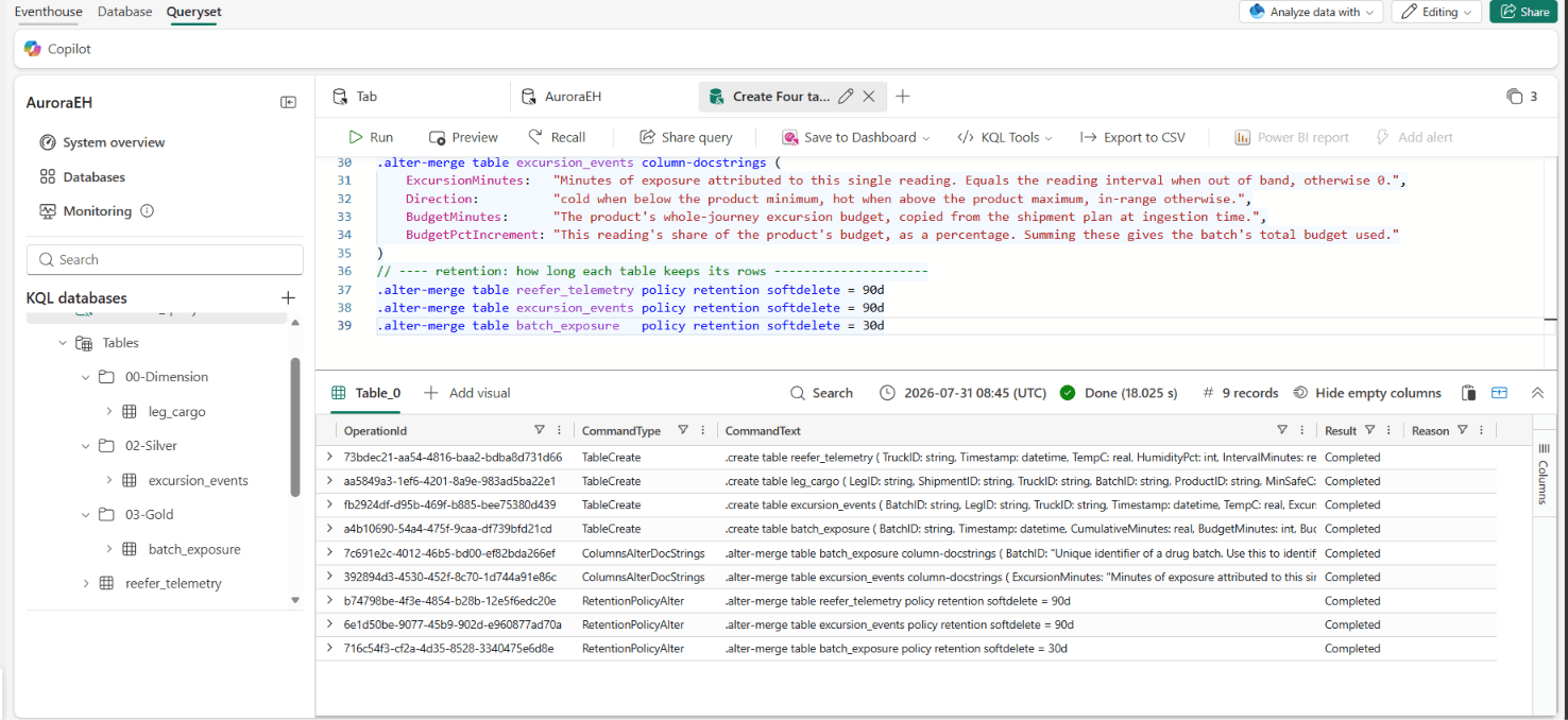
The reefer_telemetry row says Completed even though that table already exists — its declaration here matches what the eventstream wizard built in 2.6, so Kusto accepts it and changes nothing. The other three tables are new.
"Changes nothing" includes the folder. Refresh the Tables node and the three new tables sit in their folders while reefer_telemetry stays loose at the top, because folder and docstring only apply when a table is actually created. Nothing is wrong. If the untidiness bothers you:
.alter table reefer_telemetry folder "01-Bronze"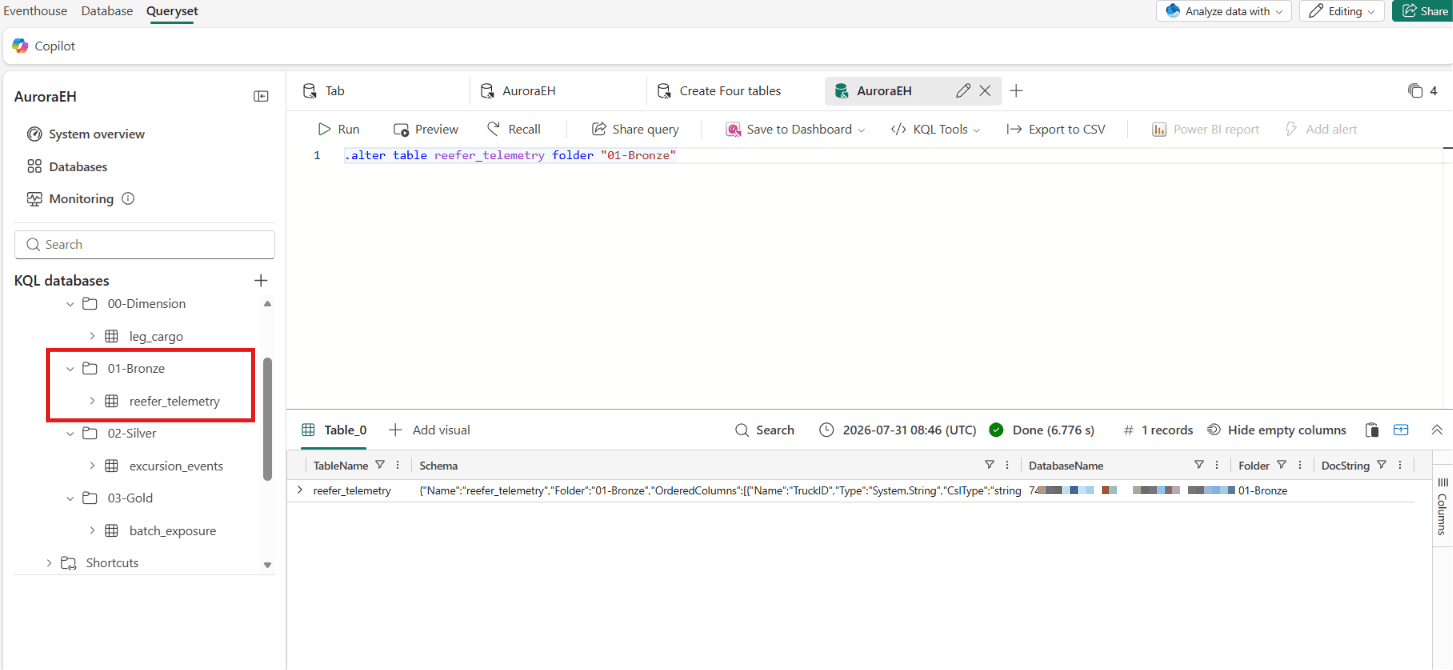
Refresh the Tables node when you are done. The three new tables sit in their folders, and if you ran the tidy-up command, all four do: 00-Dimension, 01-Bronze, 02-Silver, 03-Gold.
3.2 Load the shipment plan
Why: a truck's sensor reports one thing, how cold it is inside. It has no idea which drug batches are aboard, and no idea what temperature any of them needs. leg_cargo answers both questions, and it is the difference between a number and a verdict:
| The same reading, 9.2°C at 14:15 | Becomes |
|---|---|
Without leg_cargo | A number |
With leg_cargo | "An insulin batch aboard spent fifteen minutes 1.2 degrees above its ceiling." |
Where does the file come from? It is the derived one in the dataset: for every leg, for every batch riding that leg's shipment, one row that pulls together facts from three other files — the truck and time window from legs.csv, the batch and its product from batches.csv, and that product's safe band and budget from products.csv. It is the shipping paperwork, the route plan, and the product file merged into one flat list. In a real company, this is the export you would pull from your ERP or transport system.
It holds one row per leg per batch: a passenger list for cargo. One leg carries several batches, and one batch crosses several legs, so a single reading fans out to every batch aboard:
                     leg_cargo: who was aboard?           one scored row per batch
TRK-04 · 9.2°C  →    batch A (insulin, 2°C to 8°C)   →    batch A: 15 min above its ceiling
                     batch B (insulin, 2°C to 8°C)   →    batch B: 15 min above its ceiling
                     batch C (insulin, 2°C to 8°C)   →    batch C: 15 min above its ceiling
That fan-out is the whole reason this table has the shape it does, and 3.3 is where it happens.
One thing may look odd: this static table goes into the Eventhouse, the engine built for streams, not the lakehouse with the other static tables. That is deliberate. The scoring in 3.3 runs inside the Eventhouse, at the moment each reading lands, and a join can only reach tables in the same KQL database. The rule of thumb: data lives where its consumers are.
| Static data | Lives in | Because its consumer is |
|---|---|---|
| The six tables from Stage 1 | The lakehouse | The ontology in Stage 4 (in Part 2 of this series) |
leg_cargo | The Eventhouse, beside the stream | The 3.3 scoring join, which cannot reach across into the lakehouse |
In warehouse words: a small dimension table (a short reference list that describes things) sitting next to a large fact stream (the endless flow of readings). That pairing is a standard Kusto pattern, not a workaround, and it is where the 00-Dimension folder name in 3.1 comes from.
Why not send it through the eventstream, the way the notebook sends readings? Because an Eventhouse has two doors in, and each matches a shape of data:
| Data | Its shape | The door in | In the real world |
|---|---|---|---|
reefer_telemetry | Events: timestamped, unbounded, always arriving | The Eventstream from 2.2 | Real truck telematics send to the same custom endpoint; swap the notebook for sensors and nothing downstream changes |
leg_cargo | A plan: finite, changes only when someone schedules a shipment | Get data, a batch load | A small scheduled pipeline syncs it from the ERP or transport system whenever the plan changes |
A stream could technically carry the plan, but a one-time list would then need standing pipe infrastructure, and every plan row would be dressed up as an event. Match the door to the shape: events stream, plans load. In this build you run the load once by hand; in production, that pass becomes the scheduled sync.
Loading it takes one pass of the same Get data wizard as 2.6, and this time it is easier: the table already exists with declared types, so there is no type decision to get wrong. Eight steps:
-
Download the file to your machine. In the
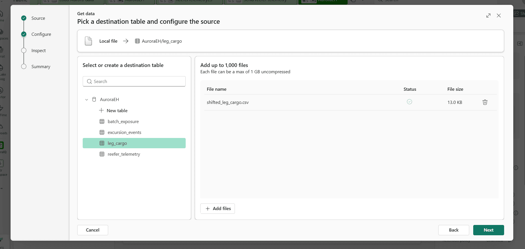
AuroraLHlakehouse → Files, right-clickshifted_leg_cargo.csvand select Download. The wizard asks for a local file and cannot browse the lakehouse. -
Open the wizard. In the
AuroraEHEventhouse, select Get data, then Local file. -
Pick the existing
leg_cargotable in the wizard's left tree, not a new one. The point is landing in the table 3.1 typed. -
Attach the shifted copy, not the original, with Browse for files. Next stays grey until a file is attached.
-
On Inspect, keep CSV and First row header ticked.
-
Check the mapping. Open the ✏️ column editor. The wizard has drafted three new
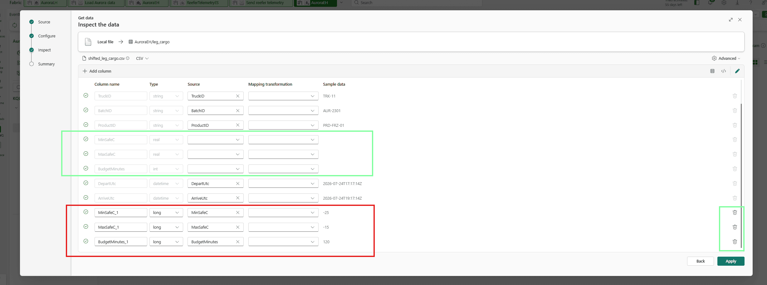
longcolumns —MinSafeC_1,MaxSafeC_1,BudgetMinutes_1— because the band values in this CSV are whole numbers (-25,2,120) and it decided they conflict with therealandintcolumns 3.1 declared. The invented rows hold the CSV sources; your real columns sit with empty Source boxes. Delete the three_1rows with the trash icon, set the Source dropdowns onMinSafeC,MaxSafeCandBudgetMinutesto their matching CSV columns, and select Apply. Skip this and every value lands in the invented columns while yours stay null, with no error anywhere.
-
Finish, once the preview shows values in every column.
-
Check the landing. Back in the queryset, in a fresh tab named
3.2 Load check:
leg_cargo
| summarize rows = count(), legs = dcount(LegID), batches = dcount(BatchID),
            missingBands = countif(isnull(MinSafeC) or isnull(MaxSafeC) or isnull(BudgetMinutes))
Four numbers come back, and each one proves something:
| Number | Proves |
|---|---|
rows = 138 | the full plan landed: one row per leg per batch |
legs = 77 | every leg of the journey is present — nothing was dropped |
batches = 61 | every batch has a truck to ride — none stranded |
missingBands = 0 | the safe bands and budgets landed as numbers; anything above 0 means null limits, and 3.3 would score nothing against them |
One honest aside before moving on. leg_cargo is the knowledge graph of this business, flattened by hand into a table so that KQL can join to it. Somebody — here, the dataset; in a real company, you — has to write out every batch-truck-leg connection as a row. The ontology in Part 2 of this series exists so that nobody has to do this flattening per question: write the connections down once, and the platform walks them for you everywhere else.
3.3 Score every reading as it arrives with an update policy
Why: you now have two tables that know nothing about each other. One holds temperatures. The other holds the shipment plan. Every question worth asking needs both.
You could join them by hand each time someone asks. That means writing the same join over and over, and getting it slightly wrong eventually.
Instead we do the join once, automatically, at the moment each reading lands. The result goes into excursion_events, where every row already knows which batch it belongs to and whether it broke that batch's limits. From here on, nobody has to remember how the join works.
The Eventhouse feature that does this is called an update policy. It comes from Kusto, and it is a rule attached to a table that says: whenever new rows arrive in table A, run this query on them and write the answer into table B. It runs by itself, forever, with nothing scheduled.
Five steps, in order. The order matters, and step 5 is the reason why:
| Step | Where | Does |
|---|---|---|
| 1. Stop the live stream | sender notebook | interrupt cell 7, wait five minutes |
| 2. Turn off streaming ingestion | queryset | a join cannot run in streaming mode |
| 3. Create the transform | queryset | the function that fans out and scores each reading |
| 4. Attach the update policy | queryset | runs the transform on everything that arrives |
| 5. Score the history | queryset | covers everything that arrived before the policy existed |
Before step 2, open a fresh tab in the queryset (+ next to the existing tabs) and name it 3.3 Update policy with the pencil icon. Everything after step 1 runs there, so the whole story of this section stays in one place.
1. Stop the live stream. Go to the sender notebook (Send reefer telemetry) and interrupt cell 7, then wait five minutes.
The wait is not superstition. Rows travel to the table in batches, and the last batch can take up to five minutes to land after the sender stops. Step 4 needs the table quiet, with nothing still in flight.
2. Turn off streaming ingestion on the raw table. The Eventstream destination you built in 2.3 set reefer_telemetry up with streaming ingestion, which writes each row the moment it arrives. An update policy that contains a join cannot run on a table in that mode. So this switch is not optional, and Microsoft is blunt about it:
To use functions with the join operator in an update policy, the streaming ingestion policy must be disabled.
Our enrichment is a join, so the raw table has to move off streaming and onto queued ingestion, which collects rows into batches before writing them. The default batch closes after five minutes.
That is a real cost, and worth understanding now rather than being surprised by later: your telemetry stops arriving instantly and starts arriving in five-minute clumps. Most of this architecture's delay comes from this one line. We add it all up in 3.5.
.alter-merge table reefer_telemetry policy streamingingestion '{"IsEnabled": false}'

.show table reefer_telemetry policy streamingingestion
Run the second command too. It prints the policy back so you can see IsEnabled really is false, rather than assuming.
3. Create the transform. The transform is the run this query half of the update policy rule above: the query the policy runs on every batch of new rows. Kusto requires it saved as a function, a named query you can call as if it were a table, which is what .create-or-alter function below does. For each new reading it finds every batch that was riding that truck at that moment, and checks that reading against each batch's own safe band. One reading in, several scored rows out, one per batch aboard.
.create-or-alter function
with (
    docstring = 'Fans one telemetry reading out to every batch riding that truck on that leg, then scores it against that product own safe band.',
    folder    = 'ColdChain'
)
ColdChain_EnrichExcursions()
{
    reefer_telemetry
    // kind=inner is required, not stylistic. See the warning below.
    | join kind=inner (
        leg_cargo
        | project LegID, TruckID, BatchID, MinSafeC, MaxSafeC, BudgetMinutes, DepartUtc, ArriveUtc
      ) on TruckID
    // Half-open window on purpose. KQL's `between` includes both ends, so a
    // reading landing exactly on a handover would be counted against two legs.
    | where Timestamp >= DepartUtc and Timestamp < ArriveUtc
    | extend IsCold = TempC < MinSafeC
    | extend IsHot  = TempC > MaxSafeC
    | extend Direction        = case(IsCold, "cold", IsHot, "hot", "in-range")
    // The reading carries its own interval, so a 15-minute recorded reading and
    // a 30-second live reading are both scored correctly by the same code.
    | extend ExcursionMinutes = iff(IsCold or IsHot, IntervalMinutes, 0.0)
    // This reading's share of the budget, computed here because this is the only
    // place that has both the minutes and the budget in hand. See 3.4.
    | extend BudgetPctIncrement =
        iff(BudgetMinutes > 0, 100.0 * ExcursionMinutes / todouble(BudgetMinutes), 0.0)
    // This column order must match excursion_events exactly.
    | project BatchID, LegID, TruckID, Timestamp, TempC, ExcursionMinutes, Direction,
              BudgetMinutes, BudgetPctIncrement
}Before wiring the transform to anything, prove it produces rows. It is an ordinary function, so you can just call it:
ColdChain_EnrichExcursions()
| summarize rows = count(), batches = dcount(BatchID)
Expect thousands of rows and 61 batches. More rows than reefer_telemetry holds is correct — that is the fan-out, one reading becoming one row per batch aboard. This check matters because of what comes next: once the policy is attached, a broken transform does not just produce bad rows, it stops ingestion.
4. Attach the update policy, which is what makes the transform run automatically from now on.
.alter table excursion_events policy update
@'[{ "IsEnabled": true, "Source": "reefer_telemetry", "Query": "ColdChain_EnrichExcursions()", "IsTransactional": true, "PropagateIngestionProperties": false }]'

.show table excursion_events policy update
The second command prints the policy back as one row. Check IsEnabled reads true and Source reads reefer_telemetry; from this moment the transform runs on everything that arrives.
IsTransactional: true means that if the transform ever fails, the raw ingestion fails with it. That sounds harsh and it is the right choice here: for a regulated cold chain, a batch quietly missing its excursion rows is far worse than an ingestion that stops loudly.
5. Score the history you already have. This is the step the whole order exists for.
The policy you just attached fires at ingestion time, for rows that arrive from now on. It never reaches back. And everything that matters in this article — the 1,812 recorded readings, AUR-2207's five frozen hours, AUR-2211's three quiet legs — arrived in Stage 2, before the policy existed. As far as excursion_events is concerned, none of it ever happened.
So score it once, by hand:
.set-or-append excursion_events <|
    ColdChain_EnrichExcursions()
Called directly like this, the function reads the whole raw table and writes every scored row into excursion_events. From this moment the two mechanisms divide the work cleanly: this command covered everything up to now, and the policy covers everything that arrives after.
This is also why step 1 stopped the stream. With rows still arriving, some would land after the policy attached but before this command ran, and be scored by both — every one of those excursions counted twice, forever, with no error. With the stream stopped and drained, the seam is clean.
Skip this step and nothing complains. The pipeline runs, the view builds, the agent answers. Every number is just missing the entire recorded journey, which is to say: wrong.
Now restart the stream. Back in the sender notebook (Send reefer telemetry), run cell 7 again. From here on, every new reading is scored automatically within a batch cycle of arriving.
Wait about five minutes, then check:
excursion_events
| summarize rows = count(), batches = dcount(BatchID), latest = max(Timestamp)
Same shape of answer as the dry run above: thousands of rows, 61 batches — and latest should now be recent and climbing, which is the update policy doing its job on the restarted stream.
3.4 Keep the running total fresh with a materialized view
Why: excursion_events now holds one scored row per reading per batch. That is a lot of rows, and none of them answer the actual question.
The question is "how many minutes has this batch used in total, across its whole journey so far?" That is a running sum, and it changes every time a reading lands.
You could add it up fresh every time somebody asks. That works, and it gets slower every day as the table grows.
Better: have the database keep the total up to date for you. The feature for that is a materialized view — a saved sum that the Kusto engine maintains by itself. When new rows arrive it adds only those, and never rescans the history. Microsoft's documentation promises exactly that:
Materialized views always return an up-to-date result of the aggregation query (always fresh).
Nothing to schedule, nothing to monitor.
One rule to work around first
There is a catch, and the workaround for it is the neatest thing in this build. Understanding it now makes the query below read effortlessly.
A materialized view can read only one table. Ours reads excursion_events. So it cannot reach across to leg_cargo to look up what a batch's budget was, which means it cannot work out a percentage. A percentage needs the total and the budget, and the view can only see one of them.
The fix was to move that work earlier, and it already happened. The update policy in 3.3 had both numbers in hand at the moment it scored each reading, so as well as the minutes it stored that reading's share of the budget, as a percentage. A reading worth 15 minutes against a 120-minute budget stored 12.5.
Now the view just adds those shares up, the same way it adds up the minutes. No second table needed.
This works because a percentage of a fixed budget is a straight multiplication, so adding the shares gives exactly the same answer as dividing the total at the end:
(15 + 30 + 45) / 120        = 75%
12.5% + 25% + 37.5%         = 75%
Same number, but the second way only ever looks at one table. The view stays legal, and the engine keeps it fresh.
Create the view
A fresh tab named 3.4 Materialized view holds this whole step: the create, its two health checks, and the first read.
.create materialized-view with (
    backfill = true,
    docstring = "Running cold-chain exposure per drug batch across every leg of its journey. Always fresh."
)
BatchExposureMV on table excursion_events
{
    excursion_events
    | summarize
        CumulativeMinutes = sum(ExcursionMinutes),
        HotMinutes        = sumif(ExcursionMinutes, Direction == "hot"),
        ColdMinutes       = sumif(ExcursionMinutes, Direction == "cold"),
        BudgetUsedPct     = sum(BudgetPctIncrement),
        FreezeEventCount  = countif(Direction == "cold" and ExcursionMinutes > 0),
        BudgetMinutes     = max(BudgetMinutes),
        LastReading       = max(Timestamp)
      by BatchID
}
Reading it now: CumulativeMinutes is the sum of minutes, BudgetUsedPct is the sum of shares from the trick above.
Two details deserve a look. backfill = true tells the engine to build the view over the rows already in excursion_events — the whole history you scored in 3.3. Leave it out and the view covers only rows arriving from this moment on, and the entire recorded story is quietly excluded.
And FreezeEventCount is counted, never budgeted. A frozen vial is destroyed, so there is no such thing as "8% of your freeze allowance used". Giving freezing its own column means it can have its own rule in Stage 6 (in Part 2 of this series), which matters because the operations agent cannot combine two conditions with AND.
Confirm it built and is keeping up
.show materialized-view BatchExposureMV

.show materialized-view BatchExposureMV failures
The first command returns one row describing the view. Two columns matter: IsHealthy should read true, and MaterializedTo should sit at or near your latest telemetry timestamp; it is the moment the view has caught up to. The second command lists every refresh failure the view has ever had, and here an empty result is the good result: no rows means no failures. Re-check IsHealthy whenever numbers look stale. A view that stops advancing is a silent outage: it keeps answering, just with old numbers.
Then read it, exactly as you would a table:
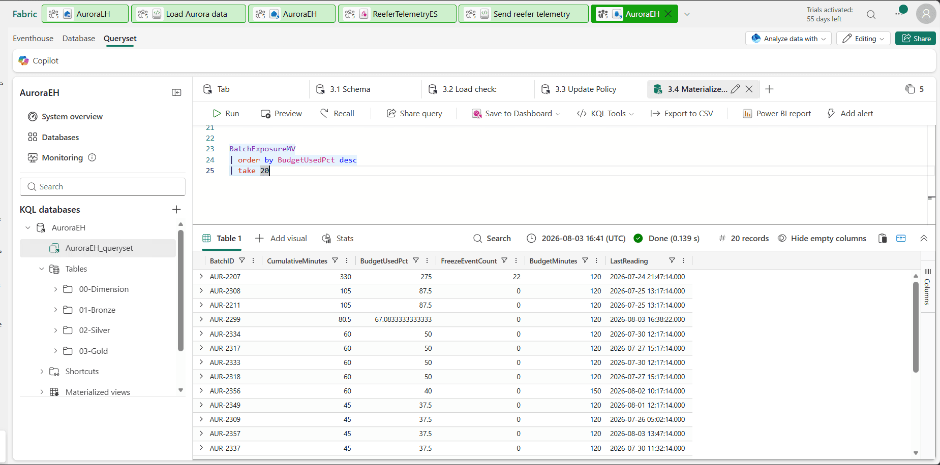
BatchExposureMV
| order by BudgetUsedPct desc
| take 20
Expect one row per batch, the top 20 of 61 shown. AUR-2207 should sit first: its 330 frozen minutes blow far past its 120-minute budget, so BudgetUsedPct is far above 100 and FreezeEventCount is above zero. AUR-2211 and AUR-2308 follow, both above 80 on their heat budgets. Those three batches are the story of this article, and 3.6 checks them against known answers.
3.5 Copy the total into a plain table
Why: this step exists only because of a product limitation. If you are wondering why we would copy a table we just built, that is the honest answer.
In Stage 6, in Part 2 of this series, you build an operations agent, the thing that watches your data and messages Teams when a batch is in trouble. It cannot read a materialized view, and Microsoft says so directly:
operations agents only support monitoring data in regular Eventhouse tables. Shortcut tables, functions, and materialized views aren't supported.
So the view we just made, the one the engine keeps perfectly fresh, is invisible to the agent that needs it most.
The fix is dull and works: a small job copies the view into an ordinary table, batch_exposure, every five minutes.
Open a fresh tab in the queryset and name it 3.5 Snapshot; the job and its check both live there. Paste the job exactly as printed — it deliberately has no blank lines inside it, because the editor would end the command at the first one, the same rule 3.1 taught:
.set-or-append batch_exposure <|
    let GraceWindow = 12h;   // keep reporting a batch this long after its last leg lands
    let AsOf        = now();
    // Only batches still in transit, or just landed. A finished journey does not
    // need a new snapshot every five minutes forever.
    let ActiveBatches =
        leg_cargo
        | where DepartUtc <= AsOf and ArriveUtc >= ago(GraceWindow)
        | distinct BatchID;
    BatchExposureMV
    // leftsemi is a pure filter: every column from the left, only the rows that
    // match on the right. No extra columns, no duplicated rows.
    | join kind=leftsemi (ActiveBatches) on BatchID
    | extend Timestamp = AsOf
    | extend BudgetUsedPct = round(BudgetUsedPct, 2)
    | extend CumulativeMinutes = round(CumulativeMinutes, 2)
    | extend FreezeEventCount = toint(FreezeEventCount)
    // Ingestion matches columns BY POSITION, not by name. This order must equal
    // batch_exposure's column order or the values land in the wrong columns.
    | project BatchID, Timestamp, CumulativeMinutes, BudgetMinutes, BudgetUsedPct, FreezeEventCount
Notice what that job does not do. It does not recompute anything, and it does not touch the raw readings. It reads a total the engine already maintains and writes it down somewhere the agent is allowed to look.
Run it once now, and confirm the copy landed:
batch_exposure
| summarize rows = count(), batches = dcount(BatchID), asOf = max(Timestamp)
Rows appear, and asOf is the moment you ran the command. That is one snapshot, and one is enough for everything in this article.
The operations agent in Stage 6 needs a fresh snapshot every five minutes, so something has to run this command on a timer. Part 2 of this series builds that: a small scheduled notebook named Refresh batch exposure that calls the KQL database from Python, scheduled from the notebook's Run menu. Fabric's scheduler accepts any recurrence from 1 to 720 minutes, and five matches the agent's own fixed evaluation cycle. The working cell is shown in Part 2, where the agent first needs it. Until then, the manual fallback is fine: re-run the command above whenever you want a fresh snapshot.
3.6 Prove it worked
Why: everything built in this stage can be wrong without telling you.
A join that quietly drops rows returns a result. A wrong type returns zero instead of an error. A view that never refreshed still answers. None of these turn anything red. The only way to know the pipeline is right is to ask it questions you already know the answers to.
Every expected number below comes from a verification script that ships beside the dataset in the project files repo: run node verify-pharma-data.mjs in that folder and it does the same arithmetic in Node over the source CSVs. You do not need to run it; the expected answers are printed with each check. If KQL and the script disagree, the KQL is wrong, not the data.
Five checks, each a query you paste and an answer you already know:
| Check | Proves | Expect |
|---|---|---|
| 1. Totals reconcile | the view agrees with the raw scored rows | Match and AllMatch both true |
| 2. Fan-out | one reading became one row per batch aboard | BatchesTouched of 2 or more |
| 3. Escalation | the verdict rule, across all 61 batches | AUR-2207 FREEZE; AUR-2211 and AUR-2308 at risk |
| 4. Freeze blind spot | a batch destroyed by cold, never once warm | HotReadings 0, ColdMinutes 330 |
| 5. Leg-by-leg total | the exposure only exists across trucks | RunningMinutes ends at 105 of 120 |
Put all five in one tab named 3.6 Verify and keep it: you will re-run these checks after the live stream has run for a while, and future you should not have to rebuild them.
1. The running total agrees with the raw rows. Add up excursion_events by hand and compare it with what the view says:
let FromView = toscalar(BatchExposureMV | summarize round(sum(CumulativeMinutes), 2));
excursion_events
| summarize FromSource = round(sum(ExcursionMinutes), 2)
| extend FromMaterializedView = FromView
| extend Match = (FromSource == FromMaterializedView)
Match must be true. Then the same test for the percentage trick from 3.4 — summed shares against direct division:
BatchExposureMV
| extend DirectPct = round(100.0 * CumulativeMinutes / todouble(BudgetMinutes), 2)
| extend ViewPct   = round(BudgetUsedPct, 2)
| extend Match     = (abs(DirectPct - ViewPct) < 0.05)
| summarize Batches = count(), AllMatch = min(Match)
AllMatch must be true across all 61 batches. If either check fails, the view is not what you think it is.
2. The fan-out happened. One reading from one truck must appear once per batch that truck was carrying:
excursion_events
| summarize BatchesTouched = dcount(BatchID) by TruckID, Timestamp
| where BatchesTouched > 1
| top 20 by BatchesTouched desc
Rows come back, with BatchesTouched of 2 or more. If this returns nothing, the fan-out never happened, and that is the classic symptom of the innerunique default join from the warning in 3.3.
3. The escalation, printed by a query. The rule from the start of this article — minutes against each product's own budget, freezing handled separately — applied to every batch at once:
BatchExposureMV
| extend Verdict = case(
        FreezeEventCount > 0,  "FREEZE - reject outright",
        BudgetUsedPct >= 100,  "budget exhausted",
        BudgetUsedPct >=  80,  "at risk",
                               "ok")
| where Verdict != "ok"
| order by FreezeEventCount desc, BudgetUsedPct desc
| project BatchID, CumulativeMinutes, BudgetMinutes, BudgetUsedPct, FreezeEventCount, Verdict
Expected: AUR-2207 marked FREEZE, and AUR-2211 and AUR-2308 at risk on their heat budgets. Sixty-one batches in, three names out, each for its own reason.
One caveat that only applies on a re-run: AUR-2299, the batch still on the road, accumulates exposure while the live stream runs, and Part 2's staged incident pushes it past 80 on purpose. Re-run this check after that demo and a fourth name appears. That is not a failure; it is the live system doing what you built it for.
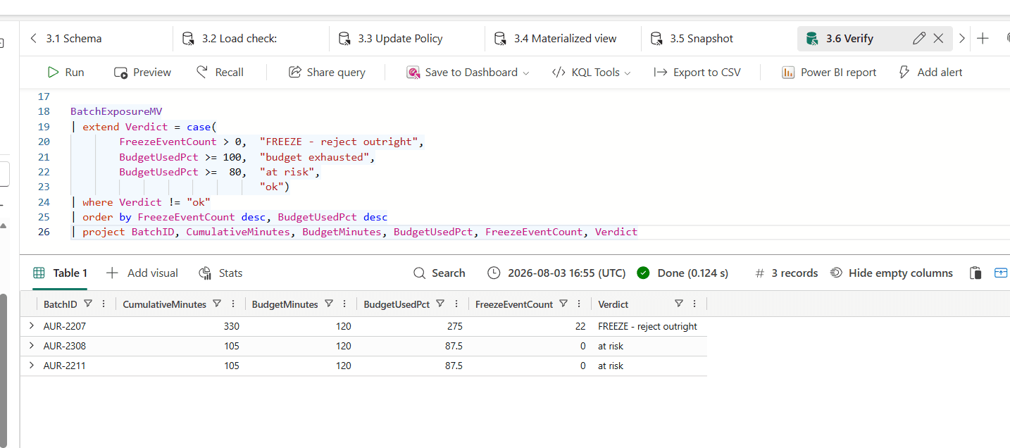
4. The freeze blind spot, proven. The batch this article opened with:
excursion_events
| where BatchID == "AUR-2207"
| summarize
    Readings       = count(),
    ColdReadings   = countif(Direction == "cold"),
    HotReadings    = countif(Direction == "hot"),
    ColdMinutes    = sumif(ExcursionMinutes, Direction == "cold"),
    ColdestReading = min(TempC),
    HottestReading = max(TempC)
Expected: HotReadings is 0, and ColdMinutes is 330. Read that twice. Not one reading above the ceiling, and every minute of a five and a half hour journey below the floor. A batch destroyed by cold, on a truck that never once got warm, invisible to every "too warm" rule anyone would normally write. That one row is the whole argument of this article, printed by a query.
5. Where the exposure happened, leg by leg. The batch nobody was adding up:
let TargetBatch = "AUR-2211";
excursion_events
| where BatchID == TargetBatch
| summarize
    LegMinutes   = sum(ExcursionMinutes),
    FirstReading = min(Timestamp)
  by LegID
| lookup kind=inner (
    leg_cargo
    | where BatchID == TargetBatch
    | project LegID, TruckID, DepartUtc, ArriveUtc
  ) on LegID
| order by FirstReading asc
| extend RunningMinutes = row_cumsum(LegMinutes)
| project LegID, TruckID, LegMinutes, RunningMinutes
Expected: three legs of 30, 30 and 45 minutes, on different trucks, with RunningMinutes ending at 105 of a 120-minute budget. No single leg looks alarming. The total is the problem, and it only exists when something follows the batch across every truck it rode. That is the answer no per-truck alarm and no dashboard of per-leg logs can give.
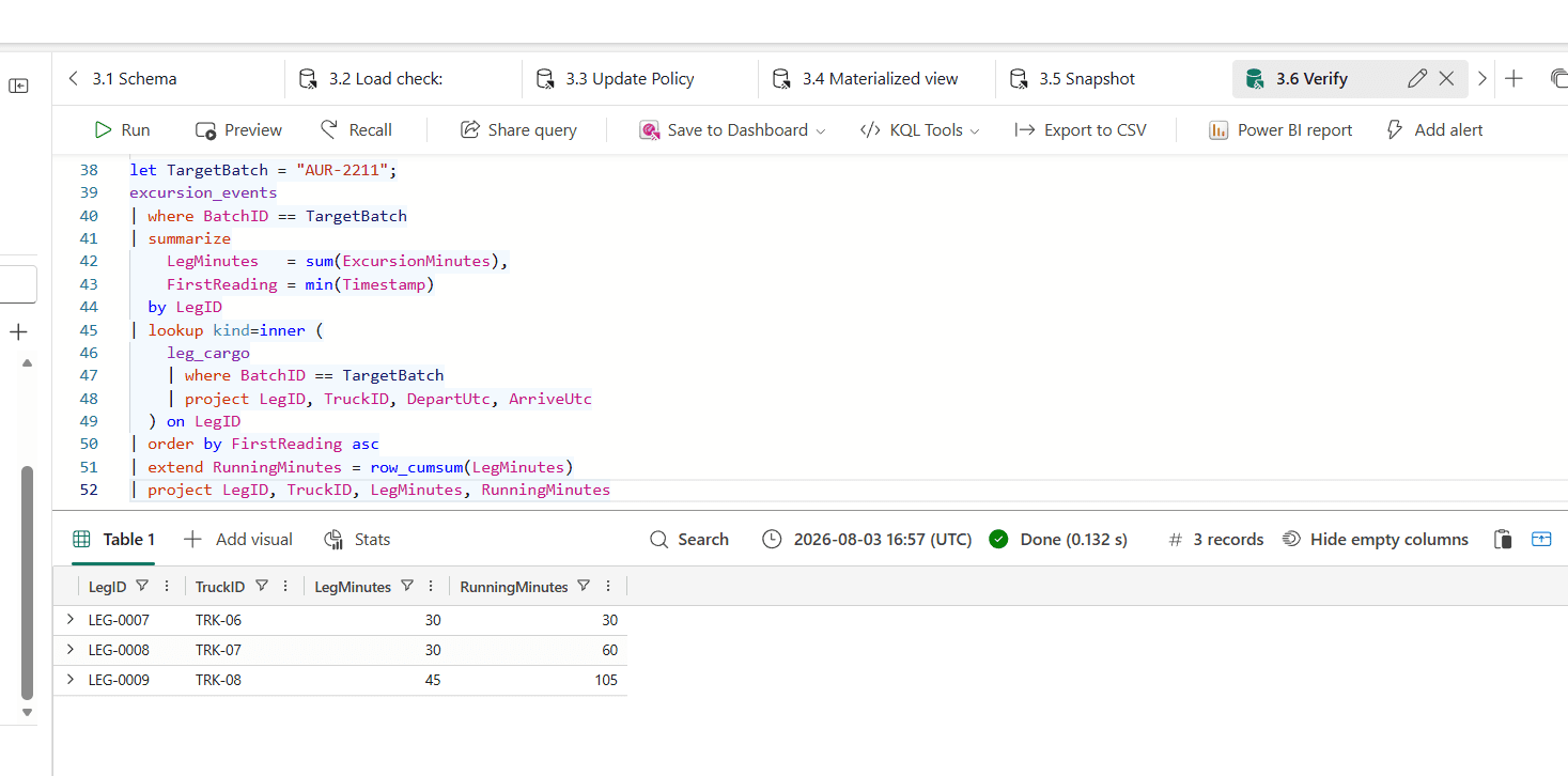
If any check disagrees and you need to dig, two places tell you why: .show ingestion failures filtered to OriginatesFromUpdatePolicy == true catches a broken transform, and the view health commands from 3.4 catch a stalled view.
What the data knows, and nobody asked
Stop and look at what exists now. Every reading is scored the moment it lands. Every batch carries a running total of the minutes it has spent outside its own product's band. The whole story of AUR-2207, five and a half hours below freezing on a truck that never once got warm, sits in a table, provable by a query.
But you had to know to ask. Every check in 3.6 was a question written by someone who already knew the answer. Nobody at a keyboard at 2am knows to ask about AUR-2207.
That is the half this article cannot finish. The data is smart now; nothing is watching it, and nothing can answer a question you have not already turned into KQL.
Part 2, publishing next, fixes both. The ontology (Stage 4) gives the data meaning an agent can traverse. The data agent (Stage 5) answers plain-language questions about batches, trucks and legs. And the operations agent (Stage 6) watches the running totals and recommends a quarantine in Teams while you are asleep.
Fresher-to-pro glossary
The plain-words phrases this article used, next to the official names you will see in the Fabric UI, the docs, and the job ads.
| Plain words in this article | Official name |
|---|---|
| The part of Fabric for data that never stops arriving | Real-Time Intelligence |
| The front door live data walks through | Eventstream; ours uses a custom endpoint source and Direct ingestion |
| The store built to hold and query that data fast | Eventhouse, and the KQL database inside it |
| The language you ask it questions in | KQL, short for Kusto Query Language; Kusto is the engine that answers |
| The editor you run queries in | KQL queryset |
| An instruction that changes the database rather than asking it a question | management command, anything starting with a dot |
| Score every reading the moment it lands | update policy |
| The running total the engine keeps fresh by itself | materialized view |
| Write each row the instant it arrives, or collect rows into batches first | streaming ingestion vs queued ingestion |
| The storage item holding files and tables in one place | Lakehouse; its tables use the Delta format, under the dbo schema |
| The raw / cleaned / finished table folders | the medallion pattern: Bronze, Silver, Gold |
| The block of computing power everything runs on | capacity; the sizes F2, F4 and up are SKUs |
| Working out column types by looking at sample data | schema inference |
| The stream of readings a machine sends about itself | telemetry |
| The machine-readable model of your business things and how they connect | ontology, a Fabric IQ item (Part 2) |
| The agent you ask, and the agent that watches on its own | data agent and operations agent (Part 2) |
| A refrigerated truck | reefer |
| Time a product spends outside its safe temperature band | excursion; the allowed total is the excursion budget |
| One stretch of a journey on one truck, site to site, like one flight of a connecting trip | a leg of the journey |